If you
do not see the menu on the left click here to see it
Before we
introduce you to programming in Stata we need to make sure you know how to
enter data into Stata and learn some basic commands along the way[1].
We will download real data in their original formats and we will proceed from
there. Once you are familiar with the basic principles of Stata we will move to
learn something about the famous "do-files". If you have some experience with
Stata you can go straight to the programming part of the course.
Stata
is a multipurpose statistical package to help you perform data analysis, data
manipulation and graphics.
There are
several ways to enter data into Stata, in this course
we will learn four different ways:
·
The
"infile' way from ASCII files using dictionary (*.dat,
*.txt)
·
The
"use' way to open Stata files (*.dta, and exporting from other stats packages like SPSS)
·
The
"quickie' way from excel (copy-and-paste)
·
The
"insheet' way from CSV files (*.csv)
·
The
"infix' way for ASCII data (you need the layout or codebook to read columns)
Depending on
your experience with Stata you should go ahead and study the following sections
at your own pace.
To start
using Stata you need two things: a properly licensed version of the software
and data.
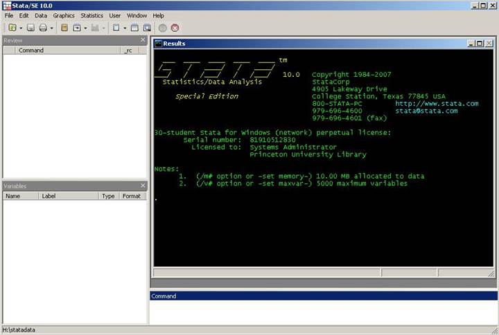
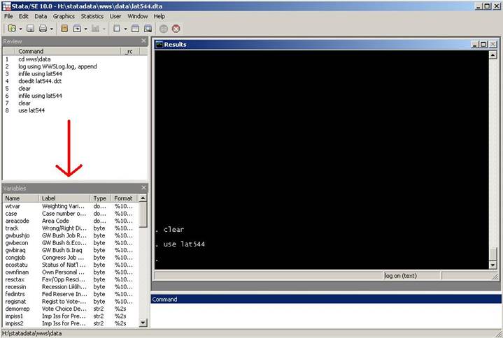
When you
first run Stata you will see this screen
With
some brief comments.
Stata has
four windows.
·
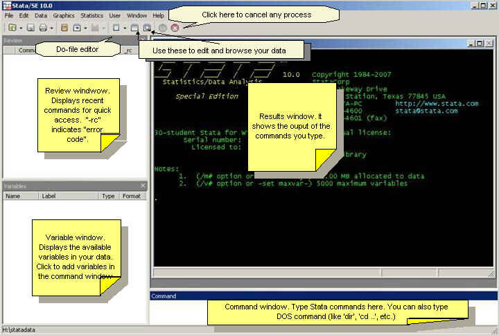
The
review window (upper left) will show the history of the commands you submit ("_rc" means error code)
·
The
results window (upper right) will show the output of every procedure you run
·
The
variables window (lower left) will show the variables of your dataset
·
The
command window (lower right) is where you type your Stata code and also DOS
commands.
You can
always use the "point-and-click" method by using the menu. We recommend
however, for most of the procedures, to use the command line.
When you work
with Stata there are three basic procedures you may want to do first: create a log file, set your
working directory, and set
the correct memory allocation for your data.
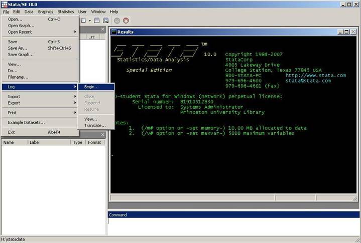
The log file
first. Go to File - Log - Begin
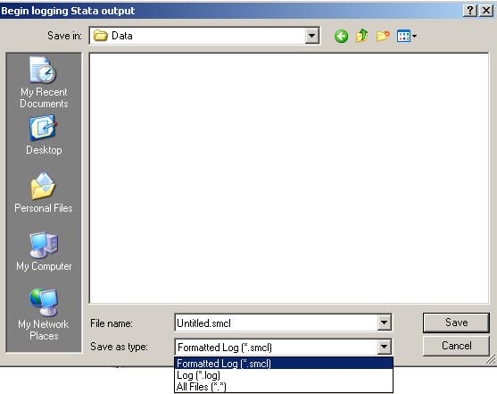
Stata will
ask you where to save the log file (you have the option of appending new output
to an existing log), choose the directory where you
want to save the log. For this course we will use the following directory in
your H: drive
H:\statadata\
I will call
the log file as Log1 and save it as a log file (which can
be read by any word processor).
Click on
"Save as type:" right below "File name:" and select Log (*.log). This will create the file called
Log1.log which can be read by any word processor or by Stata (go to File--Log
-- View). If you save it as *.smcl (Formatted Log)
only Stata can read it. It is recommended to save the log file as *.log
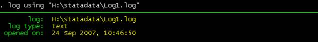
When you save
it, the Stata results window you will see something like this:
In the review
screen you will see the list of the commands you have typed so far and in the
results screen you will see the output of that command (this is useful if you
need to re-type a previous command just click on it in the review window and it
will appear in the command window)
An
alternative is to type the following code in the command window without the
"point-and-click' method (it is always recommended to work with a log file
open):
log using "H:\statadata\Log1.log", append
The second thing to do is to check is your working directory. In
the command window type the following
pwd
"pwd' stands for "print working
directory'. This will show you your working
directory, which right now, in this example is H:\statadata.
![]()
You can also
type in the command window
dir
This will
show you what is in that directory (good old DOS command).
o change directory type in the command
window
cd H:\statadata\
![]()
You can see
your current directory by looking at the lower left of the Stata screen.

The third step is to set the necessary memory allocation.
In the
picture above you can see in green letters after "Notes:" that the memory
allocation is 10 mb. This will be enough for a medium
size database but sometimes you may need more memory space to store your
dataset.
To determine
the size of your dataset follow the formula:
Size (in
bytes) = (8*Number of cases or rows*(Number of variables + 8))
Depending on
your Stata version and computer power, you can allocate up to around 2
gigabytes. To allocate 1 g you can type:
set mem 1g
Click here for a video
demonstration of these first steps.
Dealing with
public opinion data
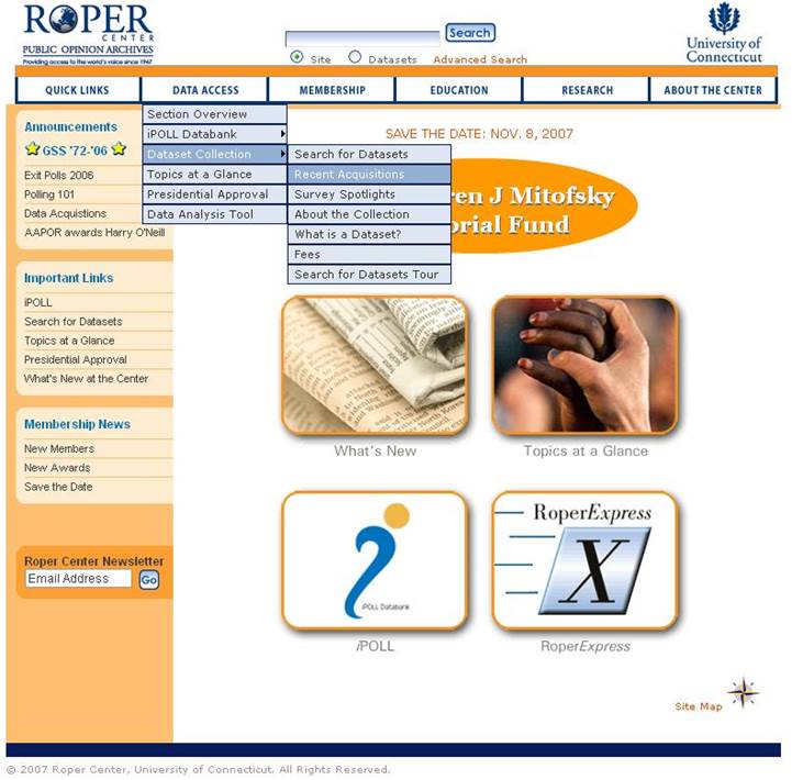
Please go to
the
http://www.ropercenter.uconn.edu/
Go to the
drop-down menu, select "Dataset Collection" - "Recent Acquisitions"
Find the
following study (if you can't find it try "search for datasets" in the same
dropdown menu):
Conducted by Los Angeles Times, field dates: April 5-9,
2007, sample: National adult [USLAT2007-544]
You can
search by using the study # USLAT2007-544.
Click on the
link for the study description. You will see links to the documentation
(codebook) and the data.
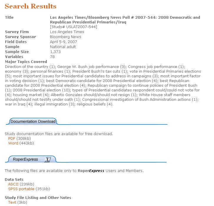
Codebook is
offered in two flavors: pdf and word, download one or the two of them if you
want.
Data is in
two formats: ASCII (*.dat, sometimes is *.txt or
*.data) and SPSS portable (which you can
open using SPSS and later save it (file-save as) as Stata this only work for
SPSS v15 or later).
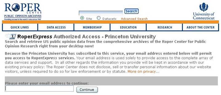
Download both
files. You will be required to enter your Princeton email (no password required
as long as you access it from the
Please save
your files in your "H:\" drive. For the course purposes we
will be working in the following directory:
H:\statadata\
Reading ASCII data
using Stata
Most data
files are in ASCII format (*.dat, *.txt, *.data,
fixed-format. It means "American
Standard Code for Information Interchange").
When dealing
with large datasets it is useful to create a dictionary file (*.dct)[2]
using the "data locations" in the codebook (you can find this section
either the *.pdf or *.doc).
A dictionary
file is useful when dealing with free format ASCII data.
The
dictionary will help you to let Stata know how many columns it has to read to
process each variable (it is like a map of your data)
To create a
dictionary file you can use notepad, wordpad or the
do-file editor in Stata (the latter highly recommended)
By "creating"
I mean open the word processor, typing the code and saving the file in a proper
format (with extension *.dct)
Let's say we
are interested in the following variables (see the codebook for the lat544
database):
[NOTE:
The following is an extract from a codebook. Codebooks differ on
how they present the layout of the data, you need to look for: variable name,
start column, end column or length, and format of the variable (whether is
numeric -and how many decimals if any- or string)]
Data Locations
Variable -- Rec -- Start -- End -- Format
WTVAR -- 1 -- 1 -- 7 -- F7.2
GWBUSHJO -- 1 -- 24 -- 25 -- A2
GWBECON -- 1 -- 26 -- 27 -- A2
ECOSTATU -- 1 -- 32 -- 33 -- A2
DEMORREP -- 1 -- 44 -- 45 -- A2
…
…
…
·
First
column tells you the variable name,
·
Second
column in which record is located (for more on this visit http://www.columbia.edu/acis/eds/stat_pak/stata/stata-write.html,
or http://www.stata.com/support/faqs/data/dict.html),
·
Third
column indicates where the variable starts,
·
Fourth
column "End" shows where the variable ends and the last column shows the format
of the variable (numeric or alphanumeric). For example, variable WTVAR is in
record 1, starts at column 1 end column 7, is numeric (letter "F") and has 2
decimal points.
For the lat544
data example there are two ways we can do this. One is using infix and
the other is using infile.
The easiest
way to extract ASCII data and put it into Stata is to type directly in the
command window the layout of the variables you want by using infix. Type
infix varname [start column-end
column] using mydatafile.*
For example:
infix wtvar 1-7 gwbushjo
24-25 gwecon 26-27 ecostatu 32-33 str demorrep 44-45 using lat544.dat
NOTE: If a variable is a string character you should add "str' before the variable name (not after) so Stata reads it
as string.
This is what
you will see in the output window.
![]()
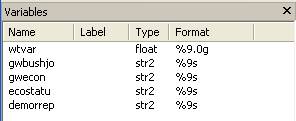
And this is
what you will see in the variables window (using either method).
You can also
open a do-file and use it to run the code (this may be useful when dealing with
a lot of variables)
infix ///
wtvar 1-7 ///
str gwbushjo 24-25
///
str gwecon 26-27 ///
str ecostatu 32-33
///
str demorrep 44-45
///
using lat544.dat
NOTE: The "///" tells Stata that all lines are part of one command
(or one line)
You can also
use infile to read fixed-format data (the
dictionary file is a bit more complex, type help infile for further details).
Using notepad
or the do-file editor the dictionary TYPE the following (do not copy-and-paste,
if you do so apostrophes need to be re-typed):
dictionary using lat544.dat {
_column(1) wtvar %7.2f "Weight"
_column(24) gwbushjo %2s "GW
Bush Job Rating"
_column(26) gwecon %2s "GW
Bush and the economy"
_column(32) ecostatu %2s "Status of Nat Econ"
_column(44) demorrep %2s "Vote
demo or rep"
}
Where
·
"dictionary
using" is the standard code to define the file as a Stata dictionary (this is "dictionary using [name of the file with the
ASCCI data] {"). Also the
curly brackets should always be in the position you see them.
·
[IMPORTANT: Always a hard return for
every line]
·
"lat544.dat"
is the name of the ASCII data.
·
_column(*)
Indicates the position where the variable starts
·
Next
write the name of the variable
·
"%7.2f"
Indicates the format of the variable (the number after % shows the number of
columns -7 in this case- and the decimal points -2 in this example-, the letter
"f" refers to a numeric fix format –an "s" will indicate a string variable
–type help format in the Stata
command window for detail information)
·
After
the format you have the option to add a variable name in quotations.
Save the file
as "lat544.dct". When saving, make sure to select
as "All files" in "Save as type:' (right below of "file name'). This is how you
create a dictionary file. To run this code you need to open Stata.
Using notepad
or the do-file editor we wrote the following dictionary:
dictionary using lat544.dat {
_column(1) wtvar %7.2f "Weight"
_column(24) gwbushjo %2f "GW Bush Job Rating"
_column(26) gwecon %2f "GW
Bush and the economy"
_column(32) ecostatu %2f "Status
of Nat Econ"
_column(44) demorrep %2s "Vote
demo or rep"
}
Save it as lat544.dct
To read data
using the dictionary we need to import the data by using the command infile.
If you want to use the menu go to File -- Import -- "ASCII data in fixed format with a
data dictionary".
With infile we run the dictionary in the
following way (for a details type help infile in the command line in Stata, also
you may want to check out infix and outfile):
infile using lat544
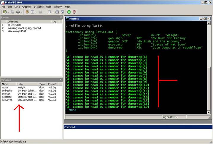
In the
"results" window you will see your dictionary and the number of observations
for your data (at the end, press the "space-bar' to finish the program). On the
lower left side in the variables window you will see the selected variables
(red arrow). In the output (results) window you will get a message that one
variable has a string character ("&"). Stata will ignore this character and
convert it to missing value.
To practice
try to import some other variables. This skill may be useful later on during
this training.
If you type browse
(in the command
line), another window will open showing your data in a spreadsheet format
Another way
to use infile is by typing directly into the command
window (you can use this method If your data is separated by comma, tabs or
space)
infile [list of variables] using [name of the datafile
including the extension]
This command
works fine when you have few variables. If one of them is string you need to
specify for example
infile string7 v1 v2 v3 using mydata.txt
In this case
v1 is a string up to 7 characters long, the other variable v2 and v3 are
numeric which is the default.
Sometimes
your data has a more complicated structured where cases are in more than one
row:
Example of a dictionary file when you have more than one
record:
dictionary using tree.dat {
_lines(3)
_line(1)
_column(1) idnum %4f
_column(5) treetype %2f
_line(2)
_column(5) soilphn %3.2f
"Soil PH - North Side"
_column(8) soilphe %3.2f
"Soil PH -
_column(11) soilphs %3.2f
"Soil PH - South Side"
_column(14) soilphw %3.2f
"Soil PH -
_line(3)
_column(5) height %5.1f
_column(10) circ %5.1f
}
Source: http://www.columbia.edu/acis/eds/stat_pak/stata/stata-write.html
Save
the dictionary with extension *.dct [for example mydictionary.dct]
Run
it by typing:
infile using mydictionary
Reading ASCII data using SPSS
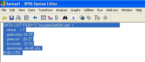
If you get
your data in ASCII format and a setup file for SPSS (with extension *.sps) you need run SPSS, go to file -- open -- syntax, find and open the *.sps. A SPSS text editor will open (it is called "syntax',
work the same way as "do-files' for Stata), you will see something like this:
…
…
…
…
DATA LIST FILE="path to
data" /
wtwar 1-7
gwbushjo 24-25
gwecon 26-27
ecostatu 32-33
demorrep 44-45 (A).
EXECUTE.
In "DATA LIST
FILE' write the path to you data with the full name of the dataset (including
the extension)
…
…
…
…
DATA LIST FILE="C:\mydata\lat544.dat" /
wtwar 1-7
gwbushjo 24-25
gwecon 26-27
ecostatu 32-33
demorrep 44-45 (A).
EXECUTE.
NOTE: The "(A)"
means that "demorrep' is a string variable. Alto
notice the dots at the end of each
command.
Select all
and click on ![]() to run it.
to run it.
In the data
window you will see your data.
If the data
is already available in a statistical package format other than Stata, it is
easier to use that format (providing you have the software) and save it or
export it to Stata. This has the advantage of including the variable labels
and, in some cases, the value labels of the data. You can also use DBMS/Copy (click
here to learn how to use it)
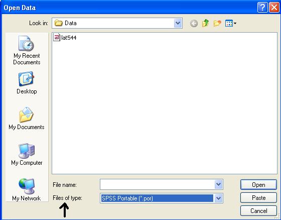
Assuming that
you have SPSS, go ahead and open the file by double clicking on lat544.por or by opening SPSS and using
the menu:
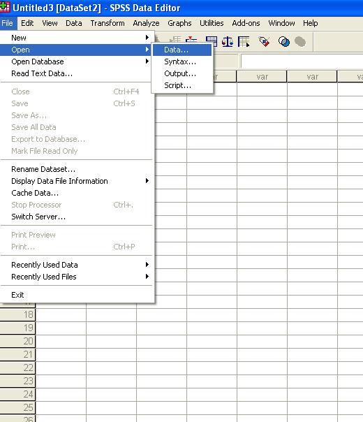
Change the
"file of type' to "SPSS Portable (*.por)", select the
file and click "Open"
Once in SPSS
you can save the data as Stata format. In SPSS go to File à Save As, the following screen will
comes up:
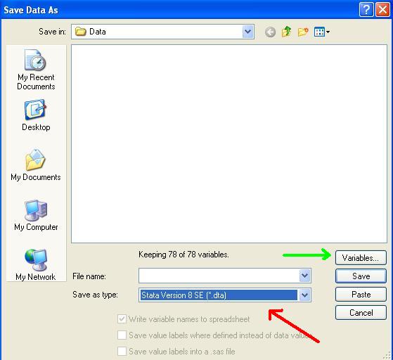
Following the
red arrow select from the list the latest version of Stata (or the
version you are working with). As an option, you can select the variables you
need by clicking in "Variables" (green arrow).
For now let's get the whole dataset.
Save the data
as lat544 and click "Save". The data will be
exported as lat544.dta
Going back to
Stata.
A note on the log file. you can close
the log file and continue using it later on.
To close the log, type
log close
To continue working on the same log
file type the following
log using "H:\statadata\Log1.log",
append
The option append will add new output
to your existing log file.
If you still
have your previous data from the dictionary, type
clear
This will
clear the data in memory so you can start with a new dataset
To read a Stata file, type
use lat544
or
use "C:\myfolder\mydata\lat544.dta"
You can also
use the menu to read a Stata file, go to File - Open.
The variable
window will be populated with all the variables in the dataset (with the
variable name, label, type and format)
In the
command line type browse if you want to check the data.
A new
spreadsheet-like window will come up.
Close the
window to go back to the command line in Stata (it is important to know that
when you browse
or edit your data you cannot use any of the
other four windows until you close the data editor)
Once you
have the data in Stata you can explore it by running the commands: describe, list,
summarize and codebook
In the
command window type
describe
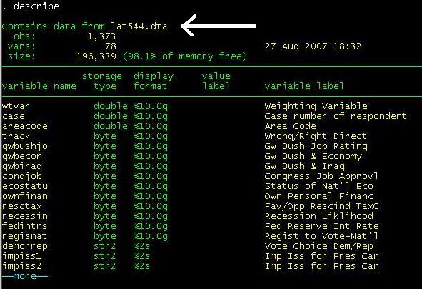
The describe command will provide you info for the
active dataset (see white arrow) and the format of the variables ("display
format"). [Hit enter or spacebar to see the rest of the list]. Type help
describe for further
details (if the "--more-- " message bugs you, type set more off)
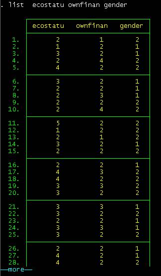
The
list command will list the data in a table
format. Since we have many variables it will be hard to read (try it, to stop
the process type the letter "q" or click on the red dot with a white "x" in the
icon row below the menu). However you can list some variables as follows:
list ecostatu
ownfinan gender
The
summarize command provides you with more information about your data. Type:
summarize
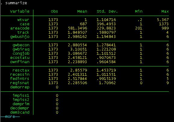
Summarize table tells you the number of cases, their
mean, sd and min and max values. Notice the "0" for
most of the variables. This means that those variables are in text (or string)
format not numeric. From the codebook we know they are supposed to be numeric.
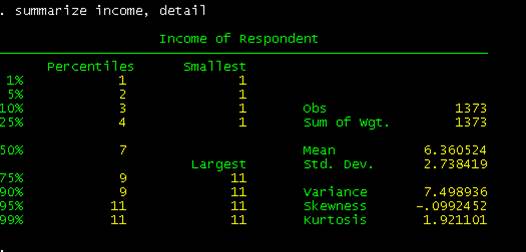
To get percentiles and other statistics you can type the
following[3]
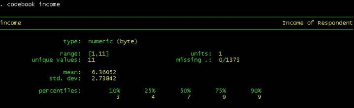
Codebook
is another useful
Stata command to explore your data, type
Type help
describe, help list, help summarize and help codebook in the command window for further
details (check also help inspect)
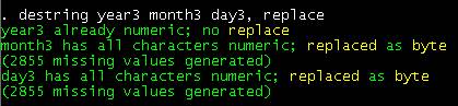
Numeric-string to numeric-numeric
To convert
numeric variables with a string (numbers in red) format into numeric we use the
command destring
destring,
replace
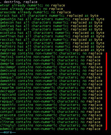
As you can
see some variables were replaced by a numeric format but others did not (see
along the red line, the screen may differ a bit from what you see) because they
contain some string characters.
Let's run a
frequency of one of these variables to see what is going on. To do this we use
the command tab

Along the red
line note the string character "&" but all the rest are numbers. We can
still convert this by using the option "ignore'. Type the following:
destring,
replace ignore(&)
Now
all variables with the string character "&" will be converted
to numeric and "&" set to missing. You
can do this with any character (a, b, x, y, *, etc).
NOTE: If destring still does not work,
here are some special cases you may want to check:
1)
Commas:
Var1
123
1,345
345
5,677
In this case type destring Var1, replace ignore(,)
WARNING: Sometimes decimals are
separated by comas, when using this make sure commas indicate thousands not
decimals. If you have decimals separated by comma type: destring Var1, replace dpcomma
2)
Spaces
Var1
123
1 345
345
5 677
In this case type destring Var1, replace ignore( )
3)
Dots
Var1
..
1 345
..
5 677
In this case type destring Var1, replace ignore(..) or sometimes there
is a space, type: destring Var1, replace ignore(.. )
You
can also destring an individual variable, type
destring
[variable(s)], replace
To
save the data go to File - Save As or type
save lat544, replace.
Continuing
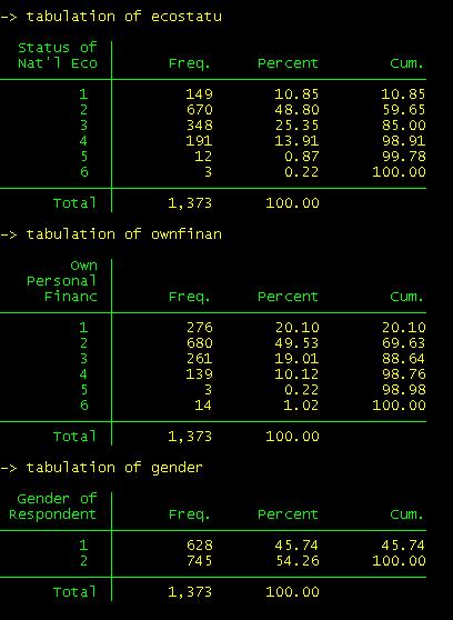
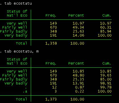
with the command tab (tabulate). Go ahead and type the following:
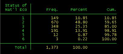
tab ecostatu
In the
results window you will se a frequency distribution
of the variable "ecostatu'.
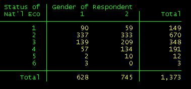
If you tab
two variables you will get a crosstabulation of those
variables (not two different frequencies)
tab ecostatu gender
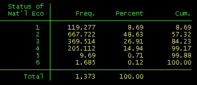
Please note
the frequency distribution and compare it with the data in the codebook. For
the variable ecostatu in the codebook
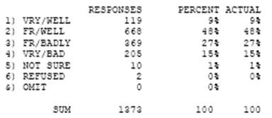
The
difference between the codebook frequencies and the Stata are the weights. The
codebook presents weighted data. So we need to weight the data to get the right
numbers. The variable "wtvar" in the dataset (first variable in
the list) contains the weights. Type the following command and see the
difference with the previous one:
tab ecostatu
[aw=wtvar]
Where "aw"
means "analytic weights' (type help weight in the Stata command line for more details)
If you want
to generate frequencies for more than one variable you use tab1 instead of tab[4]:
tab1 gwbushjo gwbecon
ecostatu
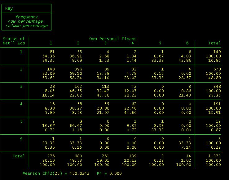
Tab
is a powerful command (type help tab in the command window for more details). For example, if
you want to test the hypothesis that two variables are independent and you want
to have row and column percentages you can use the tab command with the
following options:
tab ecostatu
ownfinan, row col chi2
By now you
might be wondering what 1, 2, 3, etc. mean. When working with public opinion
data you work mostly with categorical variables whose values most of the time
need to be labeled[5]
Stata
creates an "alternative' database for labels and you will need two commands to
label the values of the variables: label define and label values
Label define assigns a label to each category and label values assigns specific
labels to a variable
In
the case of gender, according to the codebook "1' is for "male' and "2' is for
"female'. Se we create a label called "sex' as follows. Type:
label define sex 1 male 2 female
And
we assign it to the variable gender:
label values gender sex
Type
tab
gender
and you will see the frequency distribution with the labels
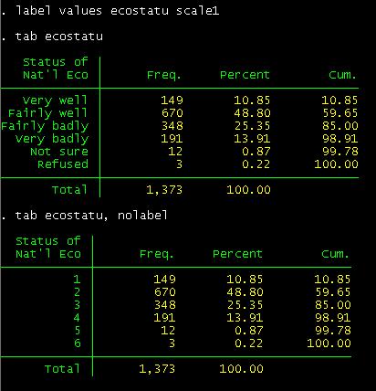
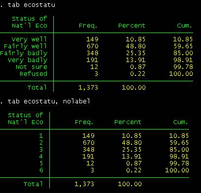
The
same thing with "ecostatu'. According to the codebook
these are the codes for the values
1 VERY WELL
2 FAIRLY WELL
3 FAIRLY BADLY
4 VERY BADLY
5 NOT SURE
6 REFUSED
Lets create a value label called "scale1'.
label define scale1 1 "Very well" 2 "Fairly well" 3 "Fairly badly" 4
"Very badly" 5 "Not sure" 6 "Refused"
And
apply it to variable "ecostatu"
label values ecostatu scale1
Type tab ecostatu
to see it with the labels.
If you do not
want to see the labels, type:
tab ecostatu, nolabel
Converting to/from missing
values
--- From
value to missing you type
For one value
mvdecode [name of the variable (type "_all' if using all variables)],
mv([# to missing])
For more than
one
mvdecode [name of the variable (type _all if using all variables)],
mv([# to missing] [# to missing] …)
or
mvdecode [name of the variable (type _all if using all variables)],
mv([# to missing]=. \ [# to missing]=.a \ [# to missing]=.b)
--- From
missing to value
For one value
mvencode [name of the variable (type "_all' if using all variables)],
mv([# assigned to missing])
For more than
one
mvencode [name of the variable (type _all if using all variables)], mv(.=[#
assigned to missing]\ .a=[# assigned to missing] \ .b=[# assigned to missing] )
Type help mvdecode or help mvencode for more details.
Example…
Using the
previous example let's say you want to convert the option 5 ("Not sure") and 6
("Refused") to missing. Type
mvdecode ecostatu, mv(5=. \
6=.a)
![]()
You get this
To do the
reverse type:
mvencode ecostatu, mv(.=5 \
.a=6)
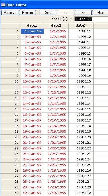
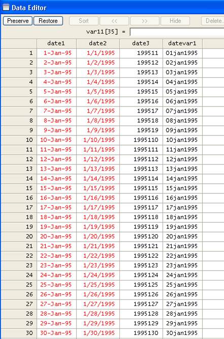
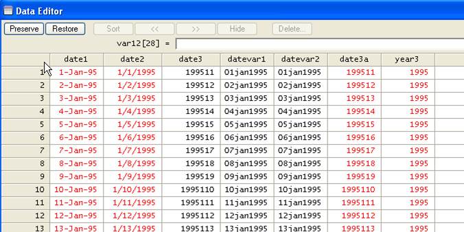
Converting text to date
Let's say you
have a date variable in either one of the following formats: "date1" and
"date2" are strings (text) and "date3" is a plain number. This data goes from
Jan 1st, 1995 to Jan 14, 2008. Neither of them is formally in date
format. We will deal with each in turn.
Summary
For "date1' use à
STATA 10 - gen
datevar1 = date(date1,"DMY", 2008)
STATA 9.2 - gen
datevar1 = date(date1,"dmy", 2008)
For "date2' use à
STATA 10 - gen
datevar2 = date(date2,"MDY", 2008)
STATA 9.2 - gen
datevar2 = date(date2,"mdy", 2008)
In both cases after creating the date variable you need
to format it as follows:
format datevar1 %td[6]
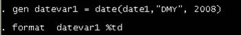
Converting "date1"
The structure
of "date1" is day-month-two digit year. For this we will use the function date()
to convert string variables into date variables. Type
STATA 10
gen datevar1 = date(date1,"DMY", 2008)[7]
STATA 9.2
gen datevar1 = date(date1,"dmy", 2008)[8]
Note, 2008
indicates that the date variable changes from 1999 to 2000. In this case it
points to the last year in the series.
then type:
format datevar1 %td[9]
"2008"
indicates the last year of the series. Date() function only recognizes year as four
digits for one century, adding 2008 forces Stata to consider the change in
centuries. For more details type help
date.
"Datevar1"
should have the same structure as "date1". Check the change in century.
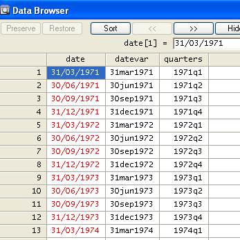
If you need
quarterly data you can transform that variable using the following:
gen quarters=qofd(datevar)
format
quarters %tq
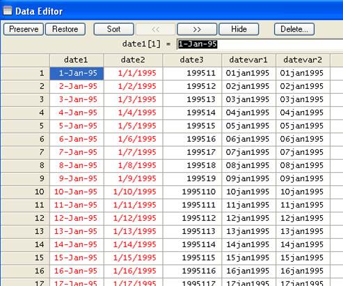
Converting "date2"
The structure
of "date2" is month-day-four digit year. For this we will also use the function
date() to convert string variables into date
variables. Type
STATA 10
gen datevar2 = date(date2,"MDY", 2008)
STATA 9.2
gen datevar2 = date(date2,"mdy", 2008)
Note, 2008
indicates that the date variable changes from 1999 to 2000. In this case it
points to the last year in the series.
then type:
format datevar2 %td
Notice that
we do not have to specify 2008 as the last year since year has four digits.
![]()
If you need
quarterly data you can transform that variable using the following:
gen quarters=qofd(datevar)
format
quarters %tq
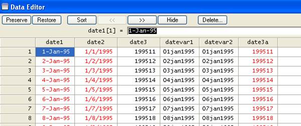
Converting "date3"
"Date3" has
the following structure: year(four digits)-month-day. It is numeric with
different lengths.
We need first
to separate its date components.
We will
generate a string variable "date3a".Type
gen date3a= string(date3,"%11.0g")
In "date3a"
year has always the first four characters, we can extract this by using the substr()
function:
gen year3=substr(date3a,1,4)
We cannot
distinguish between months and days since the rest of the characters in
"date3a" have different lengths. So we extract the rest after year. Type:
gen monthday3=substr(date3a, 5,.)
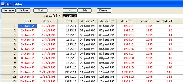
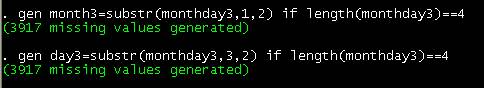
The maximum
length of "monthday3" is 4: two-digit months and two-digit days. We will
extract these first.
gen month3=substr(monthday3,1,2) if
length(monthday3)==4
gen day3=substr(monthday3,3,2) if
length(monthday3)==4
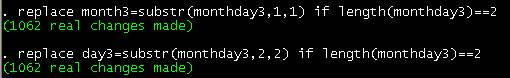
When
"monthday3" length is 2 we could be sure the first digit represents the firs nine months and the second digit the first nine days
of the month. Se can extract these in the same way
but this time we will replace the missing:
replace month3=substr(monthday3,1,1)
if length(monthday3)==2
replace day3=substr(monthday3,2,2) if
length(monthday3)==2
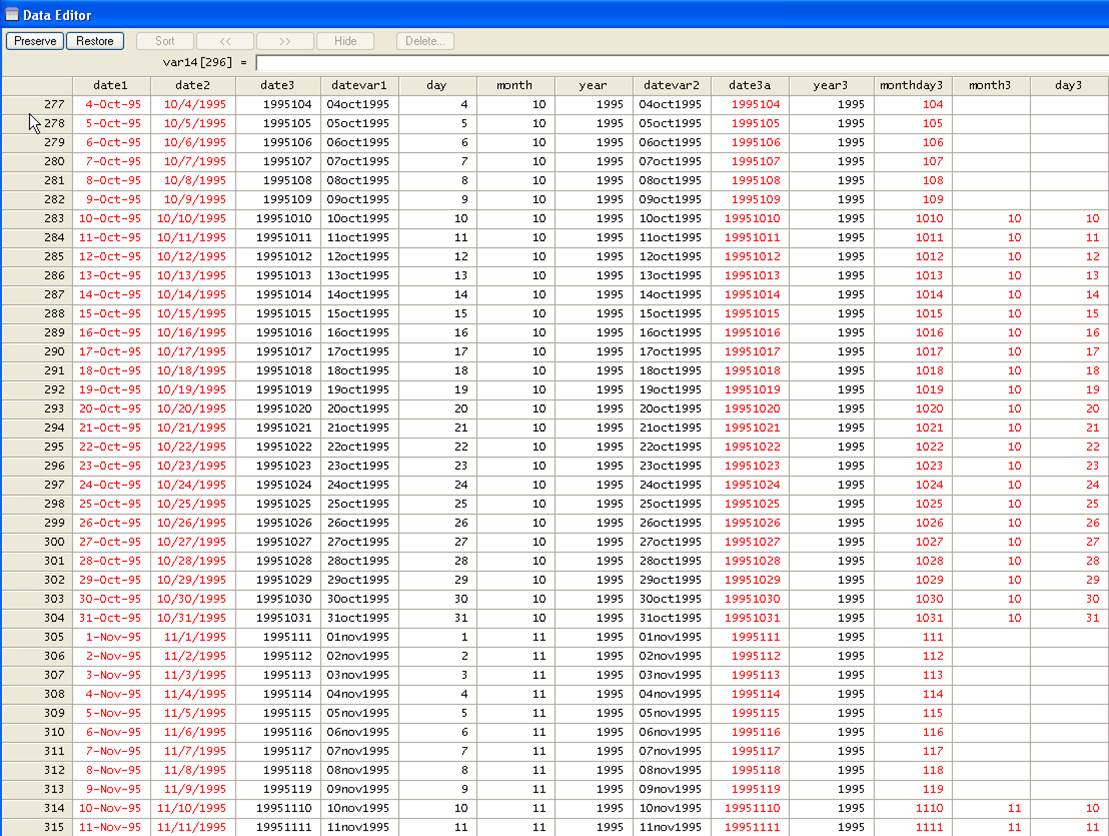
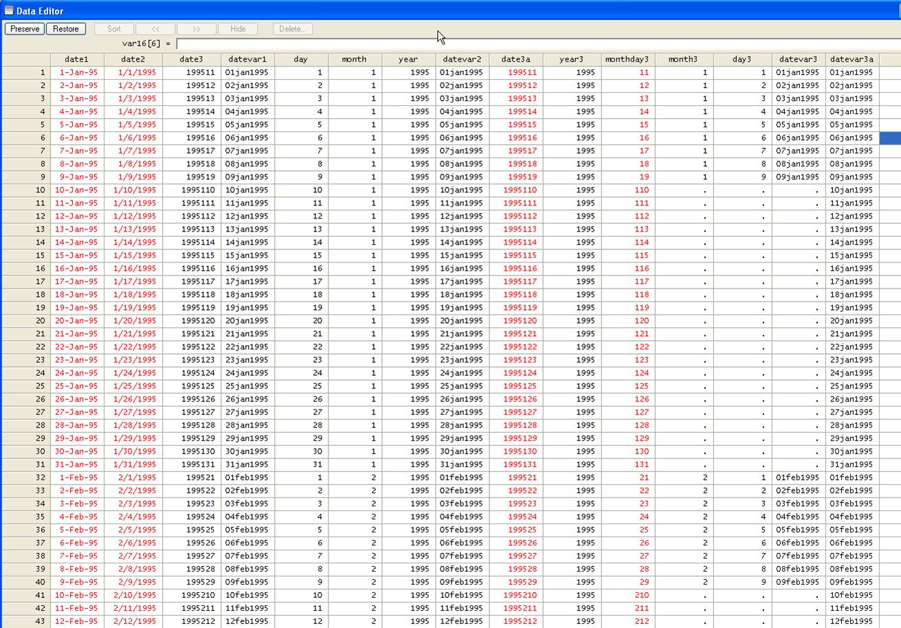
You should
have the following…

I
f you scroll down you will notice…
We will
convert these partial dates to a date variable. First we need to format
"year3", "month3" and "day3" as numbers:
destring year3 month3 day3, replace
Now we
generate the new date variable using the mdy()
function and format as %td:
gen datevar3=mdy( month3, day3, year3)
format datevar3 %td
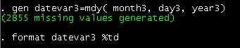
"Datevar3" is
now a partial date variable.
Notice that
one thing is the date format and another is the actual date variable. As the
following table shows, dates are a special case of a numeric variable, where
numbers are codes for dates in consecutive order. We will fill the missing
dates by simply filling in the consecutive numbers in the series.
|
This is what you see |
This is what the computer
"sees" |
|
10-Oct-95 |
13066 |
|
11-Oct-95 |
13067 |
|
12-Oct-95 |
13068 |
|
13-Oct-95 |
13069 |
|
14-Oct-95 |
13070 |
|
15-Oct-95 |
13071 |
|
16-Oct-95 |
13072 |
|
17-Oct-95 |
13073 |
|
18-Oct-95 |
13074 |
|
19-Oct-95 |
13075 |
|
20-Oct-95 |
13076 |
|
21-Oct-95 |
13077 |
|
22-Oct-95 |
13078 |
|
23-Oct-95 |
13079 |
|
24-Oct-95 |
13080 |
|
25-Oct-95 |
13081 |
|
26-Oct-95 |
13082 |
|
27-Oct-95 |
13083 |
|
28-Oct-95 |
13084 |
|
29-Oct-95 |
13085 |
|
30-Oct-95 |
13086 |
|
31-Oct-95 |
13087 |
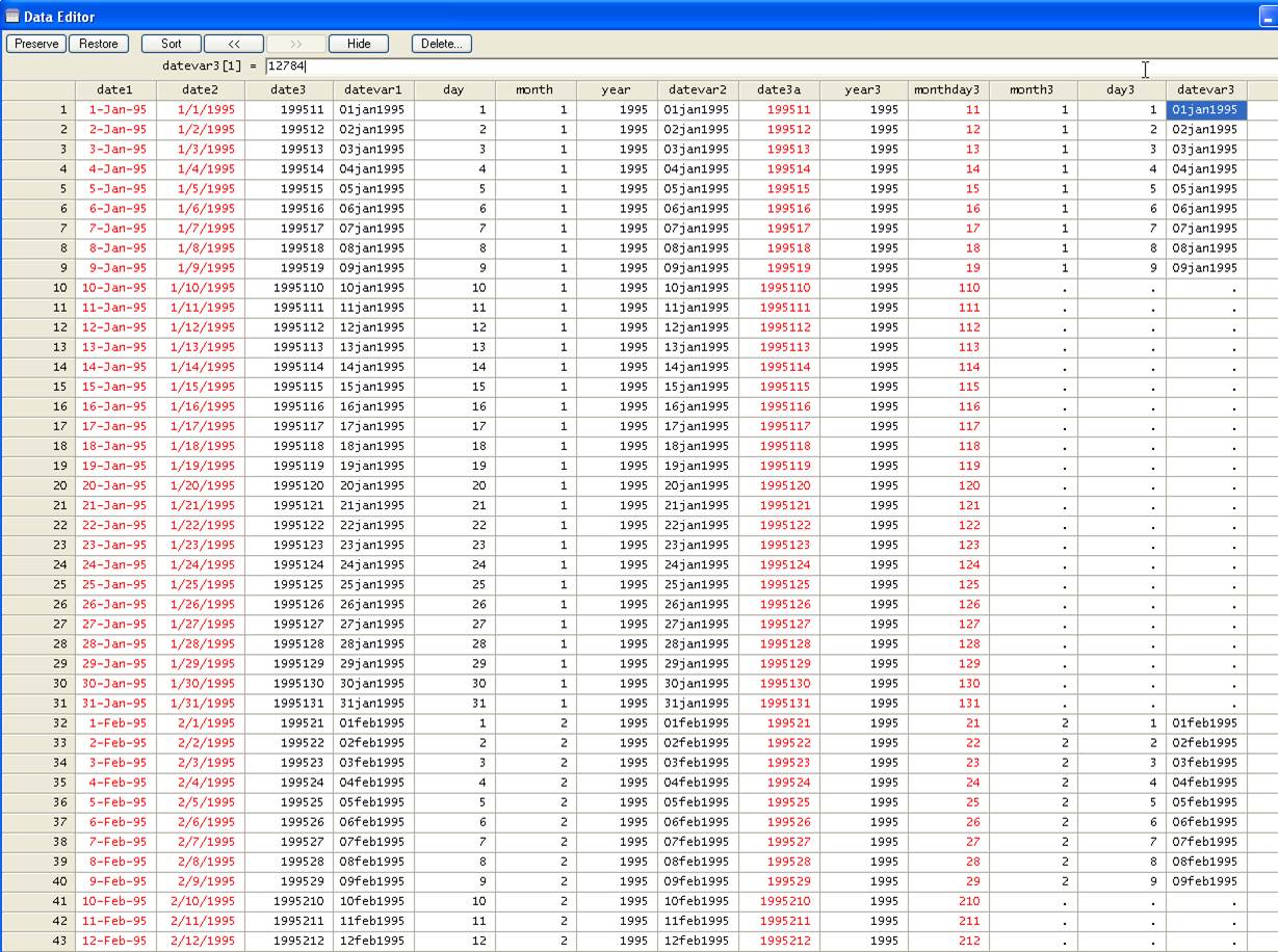
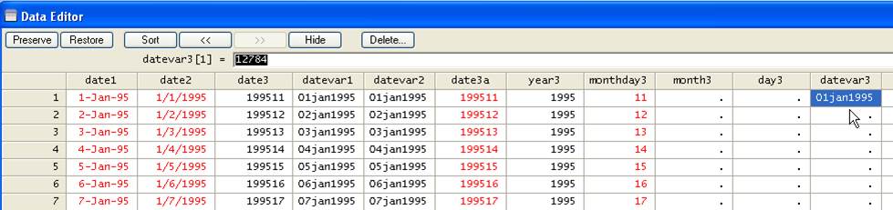
To find the
computer date codes you can use the display()and the td()
functions. For example:
display td(1jan1995)
![]()
The computer
code for Jan 1st., 1995 is 12784. If, for example, you had the first
date as missing, this is how you would replace it (this is just an example):
replace datevar3=12784 in 1
![]()
Going back to
the data. Let's make a copy of "datevar3a"
gen datevar3a=datevar3
![]()
Now we fill
in the time series:
replace datevar3a= datevar3a[_n-1]+1 if datevar3a==.
![]()

Format
"datevar3a"
format datevar3a %td
Deconstructing date
variables
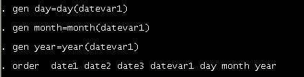
Let's say you
already have a date variable ("01jan1995") and you need to extract days,
months and years. Using date functions type:
gen day=day(datevar1)
gen month=month(datevar1)
gen year=year(datevar1)
order date1 date2 date3 datevar1 day
month year

Date
variables with day of the week
If your date
variable looks like this
Here is a
do-file to create a date variable
/*Generating
date1 */
gen date1=ltrim(subinword(date,"Monday,","
",.))
replace date1=ltrim(subinword(date1,"Tuesday,"," ",.))
replace date1=ltrim(subinword(date1,"Wednesday,"," ",.))
replace date1=ltrim(subinword(date1,"Thursday,"," ",.))
replace date1=ltrim(subinword(date1,"Friday,"," ",.))
replace date1=ltrim(subinword(date1,"Saturday,"," ",.))
replace date1=ltrim(subinword(date1,"Sunday,"," ",.))
/*Generating
date2 */
gen date2=subinstr(date1,"er","er,",.)
replace date2=subinstr(date2,"y","y,",.)
replace date2=subinstr(date2,"April","April,",.)
replace date2=subinstr(date2,"March","March,",.)
replace date2=subinstr(date2,"August","August,",.)
replace date2=subinstr(date2,"June","June,",.)
/*Generating
datevar */
gen datevar=date(date2,"MDY",2009)
format
datevar %td
You should
get the following
For further
details and other formats type[10]
help date
Time variable
For details
type help mf_date
Run this
do-file and see what happen.
set obs
100 /* Set the number of
rows to 100 */
use
"http://www.princeton.edu/~otorres/Stata/date.dta", clear
drop date1 date3
set
seed 12345
gen
hr=0+int((23-0+1)*uniform()) /*Generating a random variable with
numbers between 0 and 24 to represent hours*/
gen
min=0+int((59-0+1)*uniform())
/*Generating a random variable with numbers between 0 and 50 to
represent minutes*/
gen
sec=0+int((59-0+1)*uniform())
/*Generating a random variable with numbers between 0 and 60 to
represent seconds*/
tostring hr min sec, replace /*Convert numbers to strings*/
replace sec="0" + sec if length(sec)==1 /*Adding
"0" to single digits*/
replace min="0" + min if length(min)==1 /*Adding
"0" to single digits*/
gen
time= hr+":"+ min+":"+ sec /*Creating "time' variable as string*/
destring hr min sec, replace /*Convert strings to numbers*/
gen
double time1=hms( hr, min,
sec) /*Generating a time variable
using function hms()*/
format time1 %tcHH:MM:SS /*Formating
the time variable as time, ignore 01jan1960*/
gen
elapse= time1- time1[_n-1]
/*Creating a elapse variable in machine code*/
gen
elapsehr=hours( elapse) /*Converting elapse into hours*/
gen
elapsemin=minutes( elapse) /*Converting elapse into minutes*/
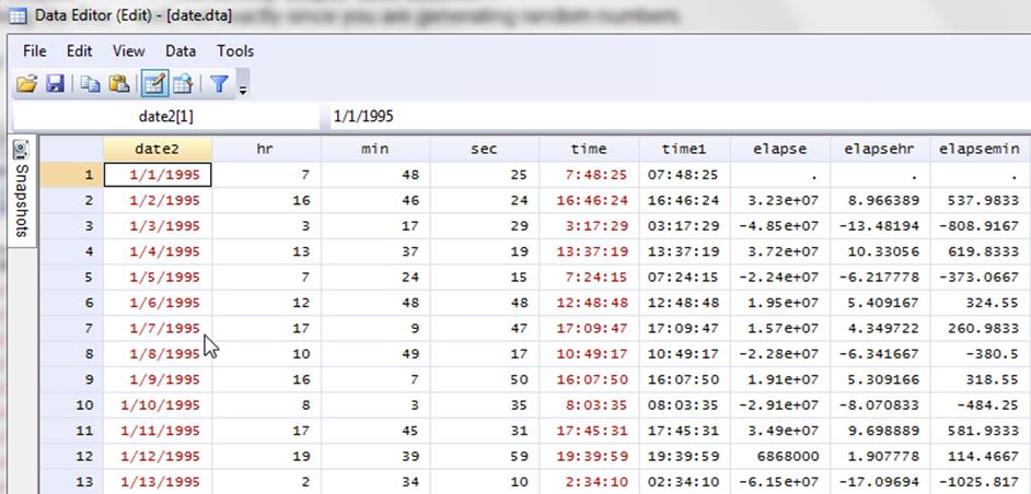
You should
have something like this… well, not exactly since you are generating random
numbers.
If you look
at the variable "elapsehr" you will notice in this example
going from the first row to the second took about 4 hrs or 237.1333 minutes.
Let's say you have "time" in the form of "hh:mm:ss" (red column above).
To separate
it into hrs, minutes and seconds as numbers (not time
variables) you can use the substr
function:
gen hour=substr(time,1,2)
gen min=substr(time,3,3)
gen sec=substr(time,6,3)
To
create a time variable from a string variable you can use the function clock:
generate double time1 = clock(time, "hms")
Then format
it as
format
time2 %tcHH:MM:SS
or
format
time2 %tcHh:MM:SSam
Combining date and time (click to see the menu on the
left)
Using the previous example
gen datevar=date(date2,"MDY",
2012) /*Date2 is a string date variable*/
format datevar %td
gen month = month(datevar)
/*Extracting month from datevar*/
gen day=day(datevar)
/*Extracting day from datevar*/
gen year=year(datevar)
/*Extracting year from datevar*/
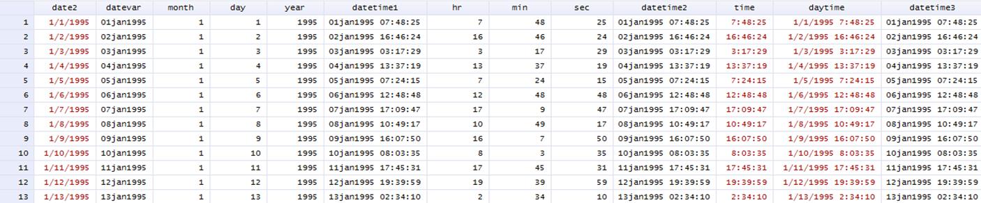
*Option 1: date
variable and time components as numbers
gen double datetime1 = dhms(datevar,hr,min,sec)
format datetime1 %tc
*Option 2: all date
and time elements as numbers
gen double datetime2 = mdyhms(month,day,year,hr,min,sec)
format datetime2 %tc
*Option 3: date and
time together as string
gen daytime = date2 + " " + time /*Creating
a date/time variable as a string*/
gen double datetime3 = clock(daytime,"MDY
hms") /*Generate day/time value from the string
version*/
format datetime3 %tc /*Format
daytime as MDYhms*/
MOVING AVERAGE FOR PANEL DATA
(click to see the menu on the
left)
Source: http://www.stata.com/support/faqs/stat/moving.html
Use the
command egenmore, you may have to install it first by
typing
ssc
install egenmore
For the lags
to work you may need to xtset your data by typing
xtset [name of panel variable] [time variable]
For example:
xtset
country year
NOTE: If you
get an error message after xtset,
click here
(page 5).
Example, for
a four year moving average type
ssc install egenmore /*If not already installed*/
use http://dss.princeton.edu/training/Panel101.dta
xtset country
year
egen moveave_x1
= filter(x1), lags(0/3) normalise
browse country year x1
moveave_x1
Where
x1 is the variable of interest. Replace x1 with your own variable.
Type help egenmore for more details.
EXTRACTING FROM
FROM A NUMERIC/STRING COMBINATION
To remove or
replace strings from var1 below use the following command (in which we are
replacing all string and special characters with nothing)
gen var2=regexr(var1,"[.\}\)\*a-zA-Z]+","")
destring var2, replace
To extract strings
from a combination of strings and numbers
gen var2=regexr(var1,"[.0-9]+","")
More info see: http://www.ats.ucla.edu/stat/stata/faq/regex.htm
Operators for
Stata's regular expression (regexr)
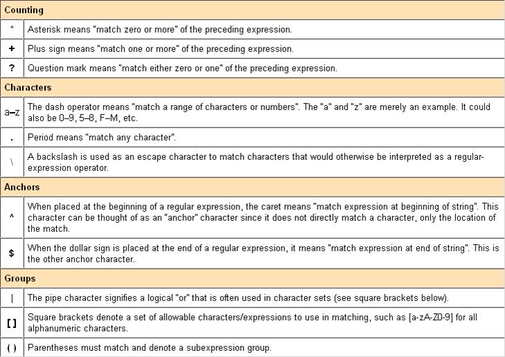
Source: http://www.stata.com/support/faqs/data/regex.html
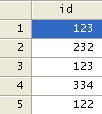
Some ids or
codes are made up from several individual codes and you may want to separate
them out. Let's assume that "id' below is composed of three different ids and
we want to create three different ids.
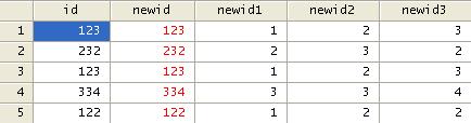
We will use the function "substr' to
separate the numbers. Steps:
1. Convert the variable from numeric to
string, type
a. tostring id, gen(newid)
2.
Use substr to extract each component
a. gen
newid1=substr(newid,1,1)
b. gen
newid2=substr(newid,2,1)
c. gen
newid3=substr(newid,3,1)
3.
Convert the individual components
back to numeric
a. destring newid1-newid3, replace
You should have something like:
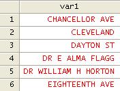
Dropping observations based on string
variables.
In the example below we want to drop observations that
contain "E.S.", we use the string function regexm, type
drop if regexm( var1,"E.S.")
> 0
Before
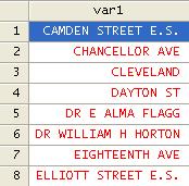
After
Dealing with
zip files within Stata
You can use unzipfile command to extract compressed data,
for example
unzipfile mydata.zip
You can also
zip file using zipfile
zipfile myzip.zip mydata.dta
For some extra info
please check:
http://www.stata.com/statalist/archive/2007-08/msg00519.html
To extract
compressed files you can also use 7-zip (freeware) available at
Or if
installed in you computer, use Winzip.
In either case,
right-click on the compressed (zip) file, select "extract to here'.
Files will
be extracted next to the zip files.
Counting groups (panel data)
(click to see the menu on the
left)
egen
count = group(panel)
Where:
"egen' = Stata command to create
special variables (type help egen
for more details)
"count' = Name of the new variable (you can change it to
something else)
"group' = Part of "egen', a
function use to create ids.
"panel' = The variable in your dataset for the panels (i.e.
country, states, companies, etc.)
Then type
summarize count
|
Variable |
Obs |
Mean |
Std. Dev. |
Min |
Max |
|
count |
70 |
4 |
2.014441 |
1 |
7 |
In this
example, the maximum number is 7 which equals the total number of panels in the
dataset
Sort variables in alphabetical order
in the variables window (click to see the menu on the
left)
Type either
order
Or
order _all, alphabetic
For more
details type
help order
To sort
cases see here
http://dss.princeton.edu/training/StataTutorial.pdf#page=45
Checking for outliers (click to see the menu on the
left)
Outliers can
change the direction of the predicted line; we need to examine the residuals.
To identify
regression residuals look at: studentized residuals,
hat values and Cook's distance
·
Cook's
distance measures how much an observation influences the overall model or
predicted values
·
Studentized
residuals are the residuals divided by their estimated standard deviation
(values >2 may be problematic).
·
Hat-points
identify influential observations on all fitted values. Go from 1/n to 1 (these
are relative to the mean hat value in the data
hat-value = (k+1)/n, k = # of predictors excluding constant)
use
http://www.ats.ucla.edu/stat/stata/examples/ara/Prestige, clear
rename educat
education
rename percwomn
women
rename occ_code
census
recode occ_type(2=1
"bc")(4=2 "wc")(3=3
"prof")(else=.), gen(type) label(type)
regress prestige education income i.type
predict yhat1 /* Predicting y*/
predict hat1, hat /*Leverage: measures the potential
leverage of Yi on all the fitted values. Pull the line towards them*/
predict res1, resid /* Getting the residuals*/
predict stud1, rstudent /* Studentized
residuals, values larger than 2 in absolute value may be problematic*/
predict cook1, cooksd /* Cook's distance, refers to values influencing the overall model */
sum hat1
local lowx =
r(mean)-r(sd)
local hix =
r(mean)+r(sd)
twoway scatter stud1 hat1 [aw= cook1], msymbol(oh)
yline(2) yline(-2) xline(`lowx') xline(`hix') || scatter
stud1 hat1 if stud1>2 | hat1>`hix', mlabels( occtitle) msymbol(i) title("Studentized residuals, Hat values and Cook's
Distance")
In the graph
below we find no significant outliers
You can see
that if you run the regression again without, the possible outliers:
MEDICAL_TECHNICIANS, ELECTRONIC_WORKERS and GENERAL_MANAGERS and plot the
fitted lines.
regress prestige education income i.type if occtitle!="MEDICAL_TECHNICIANS"
& occtitle!="ELECTRONIC_WORKERS" & occtitle!="GENERAL_MANAGERS"
predict yhat1a
twoway
lfit prestige
yhat1 || lfit prestige yhat1a
Testing interactions
using Stata 11/12 (click to see the menu on the
left)
Example 1
sysuse
auto /* Loading a
dataset that comes with Stata*/
reg
price c.mpg##i.rep78
test 2.rep78#c.mpg
test 2.rep78#c.mpg=3.rep78#c.mpg
Example2
sysuse
auto
reg
price foreign##i.rep78
test 1.foreign#3.rep78
test 1.foreign#3.rep78 1.foreign#4.rep78
test 1.foreign#3.rep78=1.foreign#4.rep78
Getting percentiles
(click to see the menu on the
left)
********Using
–summarize--
sysuse
auto /* Loading a dataset
that comes with Stata*/
sum price, detail
return list /* See saved results*/
gen pctile90=r(p90) /* Generate a variable with the 90th
percentile*/
*********Using _pctile
sysuse
auto /* Loading a
dataset that comes with Stata*/
_pctile
price, p(25 75) /*Estimating 25 and 75
percentiles*/
return list /*See the saved results
gen pctile25=r(r1) /*Creating a variable with the
25th percentile*/
gen pctile75=r(r2) /*Creating a variable with the
75th percentile*/
sum price, detail /*Checking it works*/
browse price pctile25 pctile75 /*Checking the variables*/