Lecture
1: Physics problems in early
embryonic development
(last
updated 17 March 2008)
One of the most beautiful phenomena in nature is the
emergence of a fully formed, highly structured organism from a single
undifferentiated cell, the fertilized egg. Biologists have shown that in many
cases the “blueprint” for the body is laid out with surprising speed and is
readable as variations in the expression levels of particular genes. As we try
to understand how these molecules interact to form the patterns that we
recognize as characteristic of the mature organism, we face a number of physics
problems:
How can spatial patterns in the
concentration of these molecules scale with the size of the egg, so that
organisms of different sizes have similar proportions?
What insures that the spatial
patterns are reproducible from one embryo to the next?
Since the concentrations of all
the relevant molecules are small, does the random behavior of individual
molecules set a limit to the precision with which patterns can be constructed?
Although the phenomena of life are beautiful, one might
worry that these systems are just too complicated and messy to yield to the
physicists' desire for explanation in terms of powerful general principles. For
the past several years, a small group of us have been struggling with these
problems in the context of the fruit fly embryo. To our delight, we have been
able to banish much of the messiness, and to reveal some remarkably precise and
reproducible phenomena. In particular, the first crucial step in the
construction of the blueprint really does involve the detection of
concentration differences so small that they are close to the physical limits
set by the random arrival of individual molecules at their targets. This
problem may be so serious that the whole system for constructing the blueprint
has to be tuned to maximize how much signal can be transmitted against the
inevitable background of noise, and this idea of optimization can be turned
into a theoretical principle from which we can actually predict some aspects of
how the system works (which carries us into the next lecture).
While I am very excited about the particular things my
colleagues and I are doing on this set of problems, I also hope that this lecture
will give us a chance to talk about the more general question of how one builds
bridges between general theoretical principles and the details of specific
biological systems. This theme will continue throughout the course.
In retrospect, the lecture seemed to have a logical
outline. I emphasize that what is
written here is quite rough, and should be viewed more as a guide to what was
said than as a reference text!
Some
background, and some interesting side issues
Although meant to be informal, I certainly would
appreciate feedback on these notes.
Please tell me what’s helpful, what is unclear, and where you could use
more help with background etc..
Needless to say, if there is something you find especially interesting,
I’d be happy to chat about that too!
The goal for this first half of the lecture is to
explore what we know about embryonic development in fruit flies, and to pull
out of this knowledge some physics problems (the three questions listed above)
that we think might be of general interest. We’ll start by going through what the biologists have taught
us, which really is wonderful, and then see how if we take seriously what they
tell us then we have some things which we clearly don’t understand. One way to say this is that the
biologists have given us a qualitative description of what is going on, but as
physicists we would like a quantitative theory. As we try to make qualitative ideas quantitative, two things
can happen. The first possibility
is that everything works, and what we are doing is taking the cartoons that one
sees in biology books and putting “numbers on the arrows.” This would be a good thing. But one would have to admit that if all
we do is to make quantitative versions of the biologists’ qualitative models,
then the biologists might be right to complain that we aren’t doing anything
new and we should find ways of translating our mathematical analyses back into
qualitative terms. The other
possibility, of course, is that when we try to map qualitative ideas into
quantitative ones, something seems to be missing. What’s missing might be a detail, or it might be a clue
about some general principles, and it’s hard to know which is which when we
start. I think it’s clear, though,
that we should be on the lookout for these cases where something goes wrong,
where we can’t make all the numbers fit together in a clear physical picture,
because these are the places where we have a chance to discover something
really new about the physics of life.
I hope you’ll agree that the fly embryo offers us some of these
opportunities.
We recall that even big, complicated animals like us
start out as a single cell, the fertilized egg. As the embryo develops, this one cell becomes many cells,
but importantly these cells become differentiated from one another. Cells seem to fall into discrete types,
and these types are in different locations, so this differentiation is also a
problem of spatial pattern formation.
Every cell in your body has the same DNA (assuming
nothing has gone wrong!). What
makes the different cells different is that they “express” different
genes. The genes code for
proteins, but not all of the proteins are made in all cells; the reading of the
code to make the proteins is called the “expression” of the genes. Importantly, the regulation of gene
expression is not just the flipping of a switch sometime in development, but
rather something that all cells (from neurons in our brain down to bacteria)
are doing all the time.
As physicists, when we look at the phenomena of life we
need to think about what is general and what is particular. In this lecture, we are going to look
closely at the very first stages of development and pattern formation in the
embryo of a fruit fly. Much of
what happens surely is specific to this system. But I hope you will see some general questions emerging from
these details. As noted above, at
least one of these questions (the scaling problem) is about pattern formation,
and indeed it is about a striking contrast between pattern formation in
biological vs. non-biological systems.
The other two major questions (about reproducibility and precision) are
really questions about how accurately cells can regulate the expression of
their genes, and I hope to convince you that these questions are not just
general in biological terms but also connected to some reasonably fundamental
physical problems about noise in counting molecules.
The fly embryo is an interesting model system for many
reasons. One is that there is a
well developed genetics for fruit flies (the species Drosophila melanogaster), made possible not least by
their rapid growth and reproduction.
Embryonic development itself is rapid as well, leading from a fertilized
egg to the hatching of a fully functional maggot (the larvae of flies, like
caterpillars for butterflies) within 24 hours. All of this happens inside an egg shell, so there is no
growth—pattern formation occurs at constant volume. The egg is ~1/2 mm long, so one starts
with one rather large cell, which has one nucleus. In the maggot there are ~50,000 cells. For the first three hours of
development, which will concern us most, something special happens: the nuclei multiply without building
walls to make separated cells.
Thus, for about three hours, the fly embryo is close to the physicists’
idealization of a box in which chemical reactions are occurring, with the
different molecules free to move from one end of the box to the other (perhaps
even by diffusion, although this is a more subtle question).
The duplication of the nuclei is more or less
synchronous for the first 13 divisions, which is visually quite striking. At cycle 9 or so (I don’t remember
exactly, sorry), almost all of the nuclei move to the surface of the egg, where
they form a fairly regular two dimensional lattice. With each subsequent cycle, this lattice dissolves and
reforms. You can get a sense of
all this by watching a movie here. I recommend
that you open this in a new window, since it’s a big file and you might want to
flip back and forth. This
movie was made by Thomas Gregor when he was still at Princeton (see my remarks
about collaboration, below). The fly you are looking at has been
genetically engineered so that the histone proteins in the nucleus (proteins
around which the DNA is wrapped in the chromosomes) are fluorescent, so what
you see are the chromosomes in each nucleus. As each cycle proceeds, the chromosomes bunch together,
duplicate and separate, and then one nucleus suddenly becomes two. The movie isn’t perfect, so there is
some artefactual “flashing” in the early cycles. Also, this is a mutant fly, so the stuff at the end is
weird; more about that later.
Still, I hope you get the idea.
With cycle 14, the synchronous duplication of nuclei
stops, and there is a pause while embryo builds walls between the nuclei to
make separate cells. If you stop
the action at this point and take an electron micrograph of the embryo, this is
what you see (this and the subsequent images courtesy of Eric Wieschaus). Again, the embryo is roughly ½
mm long.
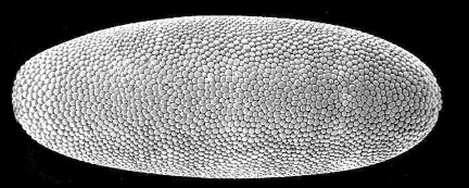
If you count, you’ll find that there are ~6000 cells on
the surface. This is smaller than
213, but that’s because not all of the nuclei make it to the
surface; some stay in the interior of the embryo, probably not by accident
since these become cells with special functions. Notice that all the cells look pretty much alike.
If instead of stopping at this point, we wait just 15
minutes more, we see something very different:
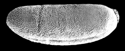
Notice that there is a vertical cleft, about one-third
of the way from the left edge of the embryo. This is the “cephalic furrow,” and defines which part of the
body will become the head. There
is also a furrow along the bottom of the embryo, which is where the one layer
of cells on the surface starts to fold in on itself so that you can have two
“outside” surfaces (think about the inside and outside of your cheek, both of
which are outside of the body from the topological point of view … we
are not simply connected!), a process called “gastrulation.” To get more of a flavor for this, you
can watch a movie of the formation
of the cephalic furrow and some perspective on gastrulation. Again I
recommend that you open this in another window. In this fly the fluorescent proteins are along the
cell membranes, so it is the boundaries between the cells that are visible. As the cells move around, these
boundaries are of course deformed in three dimensions, and this is what you see
in the movie.
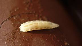
It’s not just that the embryo breaks into a head and a
non-head. In fact there are many
different pieces to the body, usually called segments. Our bodies also have segments, such as
the vertebrae along our spine. But
in insects, the segments are obvious even from the outside. Here’s an image of the fruit fly maggot
(at right), and you can see the lines on the skin, which should also be
familiar if you’ve looked closely at caterpillars (such as this lovely tiger
moth caterpillar, at left).

tiger moth caterpillar: http://www.hsu.edu/content.aspx?id=7435
fruit fly larva: http://commons.wikimedia.org/wiki/Image:Fruit_fly_larva_01.jpg
The obvious question is how the cells at different
points in the embryo “know” to become parts of different segments. The answer is quite striking, and one
of the great triumphs of modern biology.
Long before cells start moving around and making the three dimensional structures
that one sees in the fully developed organism, there is a “blueprint” that can be
made visible by asking about the expression levels of particular genes. We know which genes to look at because
of pioneering experiments first by EB Lewis and then by EF Wieschaus and C
Nüsslein–Vollhard. Lewis
identified a series of puzzling mutant flies where a mutation in a single gene
could generate flies that were missing segments, or had extra segments. It is as if the “program” of embryonic
development has sub–routines (!).
Wieschaus and Nüsslein–Vollhard decided to search for all
the genes such that mutations in those genes would perturb the formation of
spatial structure in the embryo, and they found that there are surprisingly few
such genes, on the order of 100 out the roughly 25,000 genes in the whole fly
genome. Most of these genes code for
proteins that control the expression of other genes, which means that these are
“transcription factors.”
Suppose we stop that action in the embryo at cycle 14
and measure the concentration of two of these key proteins. One way to do this is to make
antibodies against the protein we are interested in, and then make antibodies
against the antibodies, but before using the secondary antibodies we attach to
them a fluorescent dye molecule.
So if we expose the embryo first to one antibody (which should stick to
the protein we are interested in, and not anywhere else, if we’re lucky) and to
the other, we should have the effect of attaching fluorescent dyes to the
protein we are looking for, and hence if we look under a microscope the
brightness of the fluorescence should indicate the concentration of the protein
(not obvious if this relationship is quantitative; hold that question). One such experiment is shown here.
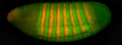
Evidently the concentration of the proteins varies with position,
and this variation corresponds to a striped pattern. The stripes should remind you of the segments in the fully
develop animal, and this is actually quite precise. Mutations that move the stripes around, or delete particular
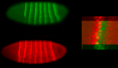
stripes, have the expected correlates in the pattern of segmentation. To illustrate this point, we can blow
up corresponding pieces of this image and the electron micrograph above,
showing the cephalic furrow:


Hopefully you can see how the furrow occurs at a place
defined by the locations of the green and orange stripes. At the moment the names of these
molecules don’t really matter.
What is important is to realize that the macroscopic structure of the
fully developed organism follows a blueprint laid out within about three hours
after fertilization, and that this blueprint is “written” as variations in the
expression level of different genes.
Furthermore, we know which genes are the important ones, and there
aren’t too many of them.
Some
background, and some interesting side issues
At this point it would be useful if you had a little
knowledge of basic molecular biology.
You need to know that DNA sequences encode proteins, and the process of
getting from DNA to protein goes in two steps: DNA is “transcribed” into messenger RNA (mRNA), and then the
mRNA is “translated” into protein.
Generating the mRNA strand is like copying the DNA strand itself, since
the mRNA is also a polymer complementary in structure to the DNA. This polymerization is catalyzed by a
molecule called RNA polymerase (RNAP), although this is an oversimplification;
in eukaryotes (cells with nuclei, including us, fruit flies and yeast), there
is a complex of roughly twenty proteins involved. Nonetheless, transcription is a polymerization reaction,
catalyzed by enzymes that “walk” along the DNA strand and leave the mRNA strand
in their wake. Translation occurs
at the ribosome, which importantly is (again, in eukaryotes) outside the
nucleus, so the mRNA needs to be exported from the nucleus in order to
function.
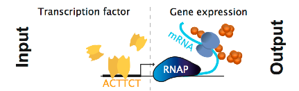
One of the basic mechanisms of regulation is to control
access of the RNA polymerase to the point at the start of the gene. In the simplest view (which probably
isn’t too bad in bacteria, although a bit more metaphorical for eukaryotes), we
can imagine controlling the expression of a gene with other proteins that
either block the RNA polymerase (and thus repress transcription) or
provide an extra place for the RNA polymerase to bind (and thus activate
transcription). These proteins are
called transcription factors, and they bind to specific sequences of DNA near
the start site for transcription; these regions of DNA that serve as control
elements are called “promoters” or “enhancers.” A schematic of all this is shown here (thanks to G Tkacik
for the figure), where we add also the ribosomes moving along the mRNA and
making protein.
I should admit that learning more about all of this,
without learning everything, isn’t so easy. Indeed, it has become more
difficult as the classic texts have become more like encyclopedias. There isn’t really a brief introduction
aimed specifically at students with a strong physics background, although many
people are struggling with this problem in their lectures. If you can get your hands on an early
edition of Watson’s Molecular Biology of the Gene, by all means read it; it is a
lovely book, with real style and personality.
Another text of great relevance is Ptashne’s book(s)
about the regulation of gene expression.
In the first instance, he focused on one model system, explored in
detail, and then briefly considered what were the general lessons to come out
of this system. In later versions,
he too tried to be more encyclopedic, but maybe less so than others.
A Genetic Switch: Gene Control and Phageλ. M Ptashne (Cell Press, Cambridge, 1986).
A Genetic Switch: Phageλand Higher Organisms (2nd edition). M Ptashne (Cell Press,
Cambridge, 1992).
A Genetic Switch: PhageλRevisited (3rd edition). M Ptashne (Cold Spring Harbor
Press, New York, 2004).
Genes and Signals. M Ptashne
& A Gann (Cold Spring Harbor Press, New York, 2002).
There are many beautiful biophysics problems lurking in
the processes of transcription and translation, even before we consider
regulation. Perhaps the most
famous of the problems is the tremendous accuracy of these reactions. The issue of how accurately genetic
information is transmitted goes back (at least) to Schrodinger’s What is
Life?
—another book very much worth reading!
Of course the great lesson of the Watson-Crick structure
for DNA is that it provides a basis for transmitting information by
complementarity: A fits with T, C
fits with G. For better or worse,
this can’t be the whole story. The
difference in binding energy between the “correct” and “incorrect” pairings
corresponds to a Boltzmann factor of ~104, when in fact the observed
accuracy is more like 1 error in every 108 base pairs, or even less
in higher organisms. In the 1970s,
Hopfield and Ninio independently realized that this problem was much more
general, and comes up in many biological processes. In effect, when cells need to link molecules together, they
seem to sort out the correct components with a reliability better than expected
from equilibrium thermodynamics, which means that they function as Maxwell
demons. This is possible, of
course, only if there is some appropriate expenditure of energy. Looking carefully at what was known
about the underlying biochemistry, Hopfield and Ninio proposed that there were
some general rules which linked energy expenditure to synthesis, and that these
served to power the Maxwell demon.
In outline, all of this has proven to be correct, although the details still
sometimes cause problems. I think
one of the most important things (which is clearest in Hopfield’s paper) is
that many different biological processes face a common physics problem, and
thus share mechanistic features which provide the solution to this probem but
otherwise look arbitrary. An important
lesson!
Kinetic
proofreading: A new mechanism for reducing errors in biosynthetic processes
requiring high specificity. JJ
Hopfield, Proc Nat’l Acad Sci (USA) 71, 4135-4139 (1974).
In the intervening 30+ years, the experimentalists have
made considerable progress. The
emergence of methods for observing single molecules in action has given us a
new window into the processes of transcription and translation, even to the
point of being able to “see” the proofreading steps as they happen. Some recent work along these lines,
very much at the forefront of a whole field of single molecule experiments, is
in the following references:
Direct observation of base-pair stepping by
RNA polymerase. EA
Abbondanzieri, WJ Greenleaf, JW Shaevitz, R Landick & SM Block, Nature 438, 460-465 (2005).
Following
translation by single ribosomes one codon at a time. J-D Wen, L Lancaster, C Hodges, A-C Zeri,
SH Yoshimura, HF Noller, C Bustamante & I Tinoco, Jr, Nature in press (2008).
Once we start to think about regulation, new problems
emerge. If we want transcription
factors to regulate particular genes, then they need to recognize something
about the sequence of the DNA near those genes, in the “promoter” regions. In one major stream of work, one uses
examples of real binding sites to try and learn what it is that these proteins
are “looking for.” One can view
this as a purely statistical problem: make up a rule that sorts the possible short DNA sequences
into two groups, one of which corresponds to binding sites and one of which
does not. But this misses the fact
that binding sites don’t have p-values, they have binding energies (!). There is a difference between saying
that a particular sequence should have a small binding energy, and that you are
not sure if it’s a binding site.
On the experimental side, several groups have developed
methods that test a transcription factor protein against, for example, all of
the promoters for the ~6000 different genes in yeast. These methods are a bit messy, and there is much discussion
of how to do the processing to clean things up and get some definite, convincing
answers. Recently, some of my
colleagues at Princeton have taken a new look at this problem, taking seriously
the physical picture that there is a binding energy characterizing the
interaction of the protein with each possible sequence. They also make use of an old idea that
this binding energy is composed of a sum of terms, one for each base pair
contact between the protein and the DNA.
They also take a very interesting view of the uncertainties in the
data: they assume that we don’t
really know how the physical binding energy relates to the measured
fluorescence signal in the experiments, and so they average over all possible
functions characterizing this relationship (more or less). Remarkably, this agnostic approach
works beautifully, even clearing up many mysteries that were left in more “fine
tuned” statistical approaches that have less physical meaning.
Precise
physical models of protein-DNA interaction from high throughput data. JB Kinney, G Tkacik & CG Callan,
Jr, Proc Nat’l Acad Sci (USA) 104, 501-506 (2007).
Although off to the side of what we want to discuss in
this lecture, all of these topics have lots of currently open problems, and I
am happy to chat with you about them (or at least point you toward people who
know more).
We have seen that the blueprint for the organism is laid
out as spatial patterns of gene expression. But how do these arise? You could imagine, as Turing did, that these patterns
reflect a spontaneous breaking of symmetries in the egg. This, for better or worse, is not how
it works. When the mother makes
the egg, she places the mRNA for a handful of proteins at cardinal points. For
example, there is a protein called Bicoid for which the mRNA is placed at the
end that will become the head, as shown in this figure.
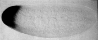
Here the embryo is stained by making DNA strands that
are complementary to the mRNA we are looking for, and attaching a label to
these synthesized DNA.
Importantly, the mRNA is attached to the end of the egg, not free
to move. Once the egg is laid, translation of this mRNA begins, and the
resulting Bicoid protein is free to move through the embryo. If we use the same trick as above and
stop the action, staining with fluorescent antibodies against the protein, we
see images like this:
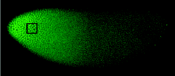
Evidently there is a rather smooth gradient in the
concentration of Bicoid protein, high at one end and low at the other. A cell sitting at some point in the
embryo thus can “know” where it is along this long (anterior-posterior) axis by
measuring the Bicoid concentration.
In fact Bicoid is a transcription factor, so it
regulates the expression of other genes.
One such gene is hunchback. If we use
the antibody staining methods to look at the concentration of the Hunchback
protein, what we see is this:

It seems as if the transformation from Bicoid to
Hunchback is almost the flipping of a switch, so that if the Bicoid
concentration is above some threshold, then Hunchback is “one,” otherwise it’s
“off.” In fact things are more
gradual, but this isn’t a bad cartoon.
There are several genes at the same level as hunchback, and again they all code for
transcription factors. Bicoid
turns all of these genes on with different thresholds, and they interact with
each other, mostly turning each other off, so that the end result is a
collection of genes which go on and off in different combinations along the
length of the embryo. These genes
in turn (along with Bicoid itself) provide input to a second layer of genes
that form the beautiful striped patterns shown above. Hunchback and its partners are called “gap genes,” because
deletion of one of these genes causes a gap of several segments in the
structure of the organism; the genes in the next layer of the systems are
called “pair rule” genes.
I think you can imagine (even without looking into all
the details) how a smooth gradient, processed by a set of threshold elements,
provides at each location a sort of combinatorial code. This code is then “read” by the next
layer of genes to produce more complex patterns. Our task, as mentioned at the outset, is to see what happens
as we try to take this qualitative scenario and turn it into something
quantitative.
Imagine that we take everything which has been said in
the previous paragraphs and formalize it in equations. In each nucleus there will be chemical
reactions corresponding to the transcription of the relevant genes, and the
rates of these reactions will be determined by the concentrations of the
appropriate transcription factors.
More equations will be needed to describe translation (although maybe
one can simplify, if, for example, mRNA molecules degrade quickly and proteins
live longer). Different points in
space are coupled, presumably through diffusion of all these molecules,
although we should worry about whether diffusion is the correct
description. Even if you’re not
sure about the details, you can
see the form of the equations.
The first problem, then, is that we have seen equations
like these before in the study of non-biological pattern forming systems such
as Rayleigh-Bernard convection, directional solidification, … . For a (very long) review, see
Pattern formation outside of equilibrium.
MC Cross & PC Hohenberg, Revs Mod Phys 65, 851-1112 (1993).
In these problems, one can observe the formation of
periodic spatial patterns which remind us of the segments in the insect and the
patterns of pair rule gene expression. The scale of these patterns, however, is
set by combinations of parameters in the equations. For example, we can combine a diffusion constant with a
reaction rate to get a length.
What happens if you put these equations in a larger box? Well, from Rayleigh-Bernard convection,
we know the answer. Recall that in
this system (a fluid layer heated from below) we see a collection of convective
rolls, sometimes in stripes and sometimes in 2D cellular patterns. Again, the length scale of the
stripes is determined by the parameters of the equation(s). If you put the whole system in a
bigger, you get more stripes, not wider stripes.
You maybe have noticed that people come in a variety of
sizes, but (for example) the fraction of the body which is head varies much
less. Almost everyone you know has
five fingers, despite variations in the size of their hands. These sound like jokes, but they are
hints about a serious problem, which can be made more quantitative for insects,
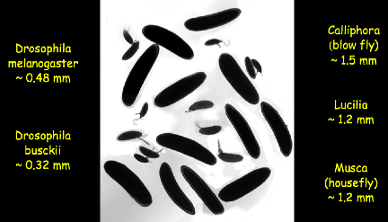
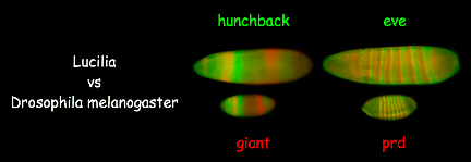
and especially for fruit flies.
There are closely related species of flies with embryos that vary in
length by a factor of five, and these embryos use molecules that are almost
identical to those in the fruit fly (you can compare the DNA sequences of the
genes). Certainly it is not
the case that embryos that are five times longer produce insects with five
times as many segments! Indeed,
what happens, to a very good approximation, is that the number of segments
stays fixed and the size of the segments scale to the size of the egg. You can see this scaling not just in
the macroscopic patterns of the developed organisms, but also in the patterns
of gene expression. These examples are from Thomas Gregor.
So, scaling is our first problem. How can a system of chemical reactions
with diffusion produce patterns that scale with the size of the container in
which they occur? Do we have to
imagine that evolution tweaks the parameters of the system slightly as we move
across flies of different sizes?
Even if this works, how does a single species deal with the variations
in length of eggs laid by the same mother?
The next problem is precision. Two neighboring nuclei along the long axis of the embryo can
certainly adopt different fates in the fully developed organism, and one can
also see that they have different patterns of expression for the pair rule
genes (although this hasn’t been checked as carefully as one might like!). One way to summarize this is that a
close look at the stripes shows that borders are only one cell wide, as in the
image below. One doesn’t see the
sort of “salt and pepper” patterns that one might if individual cells were
unsure about what to do.
What are the signals that drive these differences
between neighbors? Well, for
Bicoid we pretty much know the answer.
The concentration profile is a pretty good fit to an exponential decay
along the length of embryo, which is also what you expect if the profile
reflects a (steady state) balance between diffusion of molecules from their
source at one end of the embryo and simple first-order degradation
reactions. The length constant of
the decay is about 80 microns, and the distance between neighboring nuclei is
about 8 microns, so differences of Bicoid concentration are in the range of
~10%.
Of course we don’t know that any single step in the
readout of the Bicoid gradient is accurate to 10%, but I think this is a really
interesting possibility. Obviously
if there are billions of Bicoid molecules, noticing a 10% change is easy. But how many molecules are there? Bicoid is a transcription factor, and
it acts by binding to specific sites in the promoter region of its target
genes. Presumably the “threshold”
for turning the genes on is when about half of the relevant sites are occupied,
so the concentration scale is set by the binding energy or binding constant of
the protein to its specific site along the DNA. Protein-DNA binding has been studied in many systems, and
the usual result (including some experiments with Bicoid) is that this binding
constant is in the range of nanoMolar, which corresponds to ~0.6 molecules per
cubic micron. The nucleus is a few
microns across, so we expect that there are hundreds of molecules of Bicoid in
the nucleus at the point where the “decision” to express Hunchback (for
example) is being made. Suddenly
being sensitive to ~10% changes seems more interesting.
In fact, the number of molecules in the nucleus is not
the relevant question, but rather the rate at which molecules find their way to
their target sites along the DNA.
Long ago, in the context of bacterial chemotaxis, Berg and Purcell tried
to estimate the limits to the precision with which a system can respond to
small changes in concentration, assuming that the molecules have to arrive via
diffusion at a fixed target. Their
argument (indeed, the whole paper) is a classic of physicists’
back-of-the-envelope reasoning, also with some idiosyncrasies. You should read the original:
Physics of chemoreception. HC Berg & EM Purcell, Biohys J 20, 193-219 (1977).
I won’t repeat the arguments here (although I sketched
them in the lecture); a summary in the context of the fly embryo is given by Gregor et al (2007b). When the dust settles, given what we know about the Bicoid
concentration, typical diffusion constants for proteins in the cytoplasm, and
the size of the target, it would take many hours of averaging for the embryo to
achieve ~10% accuracy in reading out the Bicoid signal. This is implausible, since the whole
pattern forms within this time.
There seems to be a paradox here.
The problem of precision really is several
problems. First, there is the
purely theoretical question of whether the Berg-Purcell argument is
sufficiently rigorous and general to be useful in this context. Second, the Berg-Purcell limit on
precision depends on quantities such as the absolute concentration of Bicoid,
which we only estimated indirectly from the literature; it would be good to
have a direct measurement. Third,
and perhaps most crucially, we need to look carefully at a single step in the
process (e.g., the transformation from Bicoid to Hunchback) and see if this one
step really reaches the 10% level of precision; this is a question about noise
in the control of gene expression, which has been an active area recently, but
mostly in engineered model systems.
Fourth, if the system is reading out the Bicoid concentration with a precision
of ~10%, does this mean that the mother must control the absolute concentration
with similar precision in order to make sure that all embryos develop
reproducible patterns? Finally,
depending on the answers to the first three questions, we might still have a
problem to solve, and it would be nice to know the solution!
I should say that there is an overwhelming prejudice
against biological systems functioning in a highly precise fashion. Depending on how things turn out, it
might be that the fly embryo is providing an example of extreme precision, down
to the physical limits sets by the statistics of counting molecules.
As noted at the outset, a small group of us have been
working on these problems for a few years, bringing together theory and
experiment, as well as crossing the physics/biology border. The first (maybe 1.5) generation of
papers has now come out, so I will just provide pointers, with very brief
summaries.
Our first foray into the scaling problem was
Diffusion and scaling during early embryonic
pattern formation. T Gregor, W Bialek,
RR de Ruyter van Steveninck, DW Tank & EF Wieschaus, Proc Nat’l Acad Sci
(USA) 102, 18403-18407 (2005).
This work showed that, at least for inert molecules, the
diffusion equation really does describe molecular motion on the relevant length
and time scales, and that diffusion constants (perhaps not surprisingly) do not
vary significantly across embryos of very different sizes. On the other hand,
the patterns of gene expression do scale with embryo size across species, and
this scaling can be traced back to the initial anterior-posterior gradient of
Bicoid. Although there is scaling
of the spatial patterns, large and small embryos in fact develop on the same
temporal schedules. I should say
that this work was done before we had control over the issues of
reproducibility in the Bicoid profile (see below), and it would be good to go
back and do a cleaner job. The
short summary, though, is that scaling is not an emergent property of the whole
network of gene interactions, but rather a property of the Bicoid gradient
itself.
Almost everything we know about morphogen gradients has
been learned from snapshots of embryos that are fixed and stained. An alternative is to genetically
engineer flies that make a “fusion” of the protein you are interested in (e.g.,
Bicoid) and the green fluorescent protein, and this is the technical core of
the next paper,
Stability and nuclear dynamics of the Bicoid morphogen
gradient. T Gregor, EF Wieschaus, AP McGregor, W
Bialek & DW Tank, Cell 130, 141-152 (2007).
These fusion proteins are widely used in modern biology,
but for our purposes one needs to know that the fusion quantitatively
replaces the normal protein; along the way to doing this we accumulated some of
the best evidence for the linearity of the traditional antibody staining
methods, which will be important below.
Armed the green flies, one can observe (live, and at least in one color)
the dynamics of the Bicoid gradient in live embryos as they develop. An example of the resulting movies is here; as before you probably want
to open the movie in a separate window. What you are seeing are three optical sections through the
embryo, showing the complex
dynamics of Bicoid as it is repeatedly trapped and released from nuclei during
successive cell cycles.
This dynamics coexists with a constancy of the concentration inside the
nuclei, so that as the nuclei form again after one round of division the Bicoid
concentration is restored to its value at the start of the previous cycle. Photobleaching experiments demonstrate
that this constancy is the result of a rapid equilibration between the interior
of the nucleus and the surrounding cytoplasm, and the slight deviations from
constancy can be beautifully explained as an effect of changing nuclear size
during the cell cycle, balancing the dilution of molecules as the volume
increases against the increased flux as the surface area increases. Many of these results would be
understandable if the system were in an effective steady state, but the
diffusion constant of Bicoid in the cytoplasm surrounding the nuclei (which can
be estimated consistently from several different experiments) is too small to
allow establishment of this steady state in the available time. Models in which the
observed nuclear trapping is crucial to the dynamics (rather than just sampling
the surrounding cytoplasm) may also relate to the scaling problem, because the
number of nuclei is the same in embryos of different size—and hence the
local density of nuclei provides a measure of size that can be used to drive
scaling behavior.
One can also use the fusion idea more aggressively,
extracting the sequences of Bicoid from flies of different sizes and
re-inserting green versions of these different Bicoids into the Drosophila genome.
Shape
and function of the Bicoid morphogen gradient in dipteran species with different
sized embryos. T Gregor, AP
McGergor & EF Wieschaus, Dev Biol in press (2008).
The striking result is the resulting spatial profiles
are those appropriate to the host embryo, not the source of the Bicoid. Thus, the scaling problem is solved at
the level of Bicoid itself, but not by evolutionary tinkering! Rather there is something about the
environment or geometry of the embryo itself (perhaps, as suggested above, the
spacing of the nuclei) that couples the global changes in the size of the embryo
to the local dynamics. Our papers discuss models along these lines, but I don’t
think we have everything fitting together yet. I do think the theoretical problem has been sharpened,
though.
For me, interest in the fly embryo as a model system
began with the attempt to understand theoretically what defines the real limits
to the precision of signaling in biological systems. As noted above, we have an intuitive answer from Berg and
Purcell, but some work needed to be done to make this rigorous.
Physical limits to biochemical signaling.
W Bialek & S Setayeshgar, Proc Nat’l Acad Sci (USA) 102, 10040-10045 (2005);
physics/0301001.
Cooperativity, sensitivity and noise in
biochemical signaling. W
Bialek & S Setayeshgar, q–bio.MN/0601001 (2006).
Diffusion, dimensionality and noise in
transcriptional regulation. G Tkacik & W Bialek, arXiv:0712.1852
[q–bio.MN] (2007).
The result, perhaps surprisingly, is that Berg and
Purcell really did identify a lower bound on the effective noise level of a
signaling system, and this bound depends only on basic physical parameters. The (often unknown) details of the
biochemistry can add noise, but can’t lower the noise floor. This was a fun bit of statistical
physics.
With more confidence in our understanding of the
physical limits, we went back to the embryo to see how well it does:
Probing
the limits to positional information. T
Gregor, DW Tank, EF Wieschaus & W Bialek, Cell 130, 153-164 (2007).
We used the fluorescent Bicoid to make a measurement of
the absolute concentration, confirming that it is in the nanoMolar range. We then combined classical antibody
staining methods with image processing to map the input/output relation between
Bicoid and Hunchback, nucleus by nucleus, characterizing the noise in the
system (and struggling with noise in the measurements!). The noise indeed is
below 10%. To resolve the conflict
with the theoretical limits, one possibility is that nuclei, even at this early
stage of development, communicate to “agree” on the concentration of
Bicoid. If this is correct, then
the noise in the Hunchback concentration should be correlated among nearby
nuclei, and we found that this is true, with exactly the correlation length
needed to solve the noise problem.
Finally, by lining up many embryos under the microscope we could compare
the absolute Bicoid concentrations at corresponding positions, and this
reproducibility is also at the ~10% level. All of this suggests that the
reliability of a developmental decision is set by fundamental physical limits,
which is a very attractive idea.
In the same way that the initial theoretical work
provided motivation for the experiments, the experimental results have
sharpened the theoretical questions.
We’ll do more in the next lecture, but here let me point to the problem
of connecting theory and experiment more closely in the analysis of noise:
The
role of input noise in transcriptional regulation. G Tkacik, T Gregor &
W Bialek, q–bio.MN/0701002 (2007).
This work showed that not just the overall magnitude,
but also the pattern of noise in the Bcd/Hb transformation is consistent with
the idea that the dominant source of noise is the irreducible physical
randomness in the diffusion of Bcd to its targets along the Hb promoter.
I hope that I’ve been able to convey some of my
excitement about this work without overstating what we have accomplished. I think we are at the beginning rather than
an end, but perhaps with some paths now clearer. One of the crucial things that theory can do at the
interface of physics and biology is to point out which experiments are critical
in deciding among alternative directions.
But to deliver on this promise requires strong cooperative interactions
among theorists and experimentalists—not just experimental biology, but
also experimental physics. I’ve
been incredibly fortunate to have some wonderful collaborators, and to have the
whole collaboration run in a friendly and easy way, with little if any formal
structure or negotiation.
There is a lot of discussion at the moment of how to
foster interactions between physics and biology, and one should admit that
there is much frustration on both sides.
I don’t know if there are general “rules” that one can lay down for
successful collaboration. Maybe
the whole point is that, at its best, collaboration is a very intimate
relationship among individuals. In
particular, if two people (e.g., a physicist and a biologist) want to
accomplish more together than the sum of what they could do separately, then
they have to discuss with one another the things that they don’t
understand. This is hard, since
there are many forces encouraging us to hide, rather than to advertise, our
ignorance. Neither physicists nor
biologists are going to learn everything about their collaborators’ field as a
prerequisite to collaboration (it’s just like peace talks; if everybody had
agreed on terms before sitting down there probably wouldn’t have been a war).
Realistically, we may never become masters of the other field, or more
precisely we may never fully assimilate its culture, and maybe that’s a good
thing, because the novelty comes from the clash of cultures—looking at
the same phenomena, physicists and biologists ask different questions. I suspect that these thoughts on the
importance of our ignorance and the preservation of physics vs biology culture
run a bit counter to the conventional wisdom about the path to a more
homogenized quantitative biology, and I’d be happy to discuss these issues more
informally if you’re interested.
As for our particular collaboration looking at the fly
embryo, it attracted some attention, so the University newspaper ran a story about it. If you can forgive some of the pubic
relations aspects, it does give a good sense of the different personalities
involved.