CONSTRUCT SCURVE [scurve] LINE Type Parameters

Next: CONSTRUCT SCURVE [scurve] SURFACE Type Parameters Up: CONSTRUCT SCURVE Previous: CONSTRUCT SCURVE [scurve] GLOBAL X/Y/Z Type

CONSTRUCT SCURVE [scurve] LINE Type Parameters

This command is used to define a space curve which varies along a line. The curve is defined in terms of parametric distances along the line (0 to 1) and associated magnitude values. The curve may be defined as a list of position, magnitude pairs or via a function (e.g. Normal Distribution, Parabola etc.). Lists may be read in from a file or typed in at the keyboard; functions are defined interactively using a small number of control parameters.

Type	Parameters

TRIANGLE	Amplitude [Umin] [Umax]
PARABOLA	Amplitude [Power] [Umin] [Umax]
ELLIPSE	Amplitude [Umin] [Umax]
NORMAL	[Number_sd] [Umin] [Umax]
SINE	Amplitude [Umin] [Umax]
ANTISINE	Amplitude [Umin] [Umax]
LIST	FILE filename
	u,a ...

scurve	=	name of the space curve
Amplitude	=	the peak amplitude of the function
Umin	=	lower bound on function (default=0)
Umax	=	upper bound on function (default=1)
Number_sd	=	number of standard deviations (default=3)
Power	=	power of the function (default=2)
filename	=	name of ascii file containing u,a pairs
u	=	parametric distance (0 to 1)
a	=	amplitude of space curve at position u

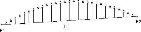
**Figure 2.21:** Definition of a line space curve
$\begin{figure} \centerline{ \psfig {figure=diagrams/scparab1.ps,width=5.0in} }\end{figure}$

Notes:

1.: Valid range
The space curve is only valid in the range between Umin and Umax.
2.: Default names
If no name is entered a default name is created, this is SCn where n is a count of defined space curves. The default name can be changed with the CONSTRUCT NAME command.
3.: Selecting portions of a space curve
The parameters Umin and Umax may be used to select a portion of one of the above functions. A common usage of these parameters is to select half of one of the functions which by default are symmetric. Setting Umin to 0 and Umax to 0.5 selects the first half of the space curve, Umin to 0.5 and Umax to 1.0 selects the second half of the space curve. The resulting space curve will be mapped to the full parametric space of the line. These parameters are also useful for reversing the sense of a space curve on a line rather than re-defining the line itself.
4.: Interaction with loads
A line space curve will multiply a load at a node, element face centroid or element centroid (depending upon the load type) by the value of the space curve at that point in space.
5.: Interaction with load masks
A line load mask will compress a line space curve so that all of the curve fits within the load mask limits. A global load mask will truncate a line space curve.
6.: Reading lists from a file
It is possible to read in long lists of space curve data from file. The file must be ascii and have one u,a pair on each line. The u,a values must be separated by either a comma or a space. The maximum allowable number of u,a pairs is machine dependent but will be at least 10000.
7.: Viewing space curves
Space curves may be viewed either by applying them to a load and using the command LABEL MESH LOADS or by using the command UTILITY GRAPH SCURVE.
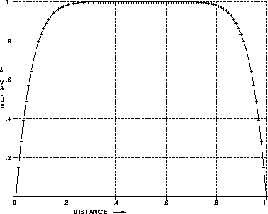
8.: The Power parameter on PARABOLIC space curves
This parameter is set to 2 by default to give the standard parabolic shape although the power parameter can be set to any even number. Setting the value to 8 gives a space curve shape which is common in boundary layer modelling.
9.: The Number_sd parameter on NORMAL space curves
This parameter is set to 3 by default and governs the number of standard deviations which are included in the curve. When set to 3 the area under this curve will be 0.997 which is useful for changing the distribution of a load without changing its total.

Examples:

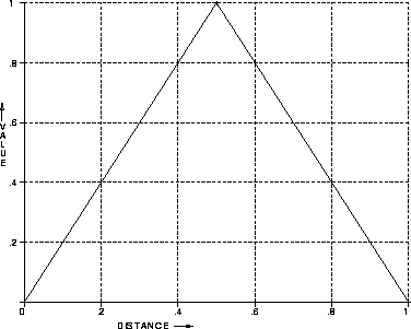
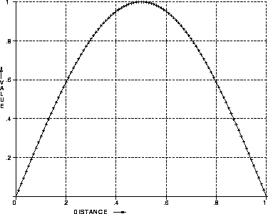
1.

CONSTRUCT SCURVE LINE TRIANGLE 1

**Figure 2.22:** TRIANGLE line space curve
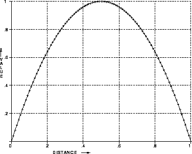
$\begin{figure} \centerline{ \psfig {figure=diagrams/scltri.ps,width=3.5in} }\end{figure}$

2.

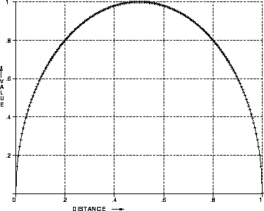
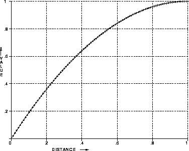
CONSTRUCT SCURVE LINE PARABOLA 1

**Figure 2.23:** PARABOLA line space curve
$\begin{figure} \centerline{ \psfig {figure=diagrams/sclpar.ps,width=3.5in} }\end{figure}$

3.

CONSTRUCT SCURVE LINE PARABOLA 1 8

**Figure 2.24:** PARABOLA line space curve
$\begin{figure} \centerline{ \psfig {figure=diagrams/sclpar2.ps,width=3.5in} }\end{figure}$

4.

CONSTRUCT SCURVE LINE ELIPSE 1

**Figure 2.25:** ELIPSE line space curve
$\begin{figure} \centerline{ \psfig {figure=diagrams/scleli.ps,width=3.5in} }\end{figure}$

5.

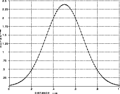
CONSTRUCT SCURVE LINE NORMAL 3

**Figure 2.26:** NORMAL line space curve
$\begin{figure} \centerline{ \psfig {figure=diagrams/sclnor.ps,width=3.5in} }\end{figure}$

6.

CONSTRUCT SCURVE LINE SINE 1

**Figure 2.27:** SINE line space curve
$\begin{figure} \centerline{ \psfig {figure=diagrams/sclsin.ps,width=3.5in} }\end{figure}$

7.

CONSTRUCT SCURVE LINE ANTISINE 1

**Figure 2.28:** ANTISINE line space curve
$\begin{figure} \centerline{ \psfig {figure=diagrams/sclant.ps,width=3.5in} }\end{figure}$

8.

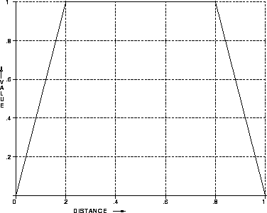
CONSTRUCT SCURVE LINE LIST 0 1 .2 1 .8 1 1 0

**Figure 2.29:** LIST line space curve
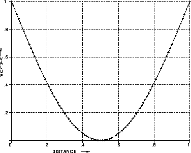
$\begin{figure} \centerline{ \psfig {figure=diagrams/scllis.ps,width=3.5in} }\end{figure}$

9.

CONSTRUCT SCURVE LINE PARABOLA 1 2 0 .5

**Figure 2.30:** Half PARABOLA line space curve
$\begin{figure} \centerline{ \psfig {figure=diagrams/sclpar3.ps,width=3.5in} }\end{figure}$

See also the following commands

'CONSTRUCT NAME'
'CONSTRUCT LMASK'
'CONSTRUCT TCURVE'
'PROPERTY ATTACH'
'PROPERTY LOAD'
'UTILITY DELETE'
'UTILITY TABULATE'

Next: CONSTRUCT SCURVE [scurve] SURFACE Type Parameters Up: CONSTRUCT SCURVE Previous: CONSTRUCT SCURVE [scurve] GLOBAL X/Y/Z Type

Femsys Limited
1st October 1999