Back to the Index
CHAPTER 1: PROBABILITY
Introduction
"Yes or no: was there once life on Mars?" I can't say. "What about intelligent life?"' That seems most unlikely, but again, I can't really say.The simple yes-or-no framework has no place for shadings of doubt; no room to say that I see intelligent life on Mars as far less probable than life of a possibly very simple sort. Nor does it let me express exact probability judgments, if I have them. We can do better.
What if I were able to say exactly what odds I'd give on there having been life, or intelligent life, on Mars? That would be a more nuanced form of judgment, and perhaps a more useful one.
1.1 Bets and ProbabilitiesSuppose my odds were 1:9 for life, and 1:999 for intelligent life, corresponding to probabilities of 1/10 and 1/1000, respectively; odds m:n correspond to probability m/(m+n.) That means I'd see no special advantage for either player in risking one dollar to gain nine in case there was once life on Mars; and it means I'd see an advantage on one side or the other if those odds were shortened or lengthened. And similarly for intelligent life on Mars when the risk is 1 thousandth of the same ten dollars (1cents ) and the gain is 999 thousandths ($9.99).
Here is another way of saying the same thing: I'd think a price of one dollar just right for a ticket worth ten if there was life on Mars and nothing if there wasn't, but I'd think a price of only one cent right if there has to have been intelligent life on Mars for the ticket to be worth ten dollars.

So if I have an exact judgmental probability for truth of a hypothesis, it corresponds to my idea of the right price for a ticket worth 1 unit or nothing depending on whether the hypothesis is true or false. (For the life on Mars ticket the unit was $10; the price was a tenth of that.)
Of course I have no exact judgmental probability for there having been life on Mars, or intelligent life there. Still, I know that any probabilities anyone might think acceptable for those two hypotheses ought to satisfy certain rules, e.g., that the first can't be less than the second. That's because the second hypothesis implies the first: see the implication rule in sec. 3 below. Another such rule, for 'not': the probabilities that a hypothesis is and is not true must add to 1.
In sec. 2 we'll turn to the question of what the laws of judgmental probability are, and why. Meanwhile, take some time with these questions, as a way of getting in touch with some of your own ideas about probability. Afterward, read the discussion that follows.
Questions
1 A vigorously flipped thumbtack will land on the sidewalk. Is it reasonable for you to have a probability for the hypothesis that it will land point up?
2 An ordinary coin is to be tossed twice in the usual way. What is your probability for the head turning up both times--
(a) 1/3, because 2 heads is one of three possibilities: 2 heads, 1 head, 0 heads?
(b) 1/4, because 2 heads is one of four possibilities: HH, HT, TH, TT?
3 There are three coins in a bag: ordinary, two-headed, and two-tailed. One is shaken out onto the table and lies head up. What should be your probability that it's the two-headed one--
(a) 1/2, since it can only be two-headed or normal?
(b) 2/3, because the other side could be the tail of the normal coin, or either side of the two-headed one?
4 "It's a goy!"
(a) As you know, about 49% of recorded human births have been girls. What's your judgmental probability that the first child born in the 21st century will be a girl?
(b) A goy is defined as a girl born before the beginning of the 21st century or a boy born thereafter. As you know, about 49% of recorded human births have been goys. What is your judgmental probability that the first child born in the 21st century will be a goy?
Discussion
1 Surely it is reasonable to suspect that the geometry of the tack gives one of the outcomes a better chance of happening than the other; but if you have no clue about which of the two has the better chance, it may well be reasonable to have judgmental probability 1/2 for each. Evidence about the chances might be given by statistics on tosses of similar tacks, e.g., if you learned that in 20 tosses there were 6 "up"s you might take the chance of "up" to be in the neighborhood of 30%; and whether or not you do that, you might well adopt 30% as your judgmental probability for "up" on the next toss.
2, 3. These questions are meant to undermine the impression that judgmental probabilities can be based on analysis into cases in a way that doesn't already involve probabilistic judgment (e.g., the judgment that the cases are equiprobable).
In either problem you can arrive at a judgmental probability by trying the experiment (or a similar one) often enough, and seeing the statistics settle down close enough to 1/2 or to 1/3 to persuade you that more trials won't reverse the indications.
In each these problems it's the finer of the two suggested analyses that makes more sense; but any analysis can be refined in significantly different ways, and there's no point at which the process of refinement has to stop. (Head or tail can be refined to head-facing-north or head-not-facing-north or tail.) Indeed some of these analyses seem more natural or relevant than others, but that reflects the relevance of probability judgments that you bring with you to the analyses.
4. Goys and birls.
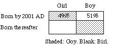
This question is meant to undermine the impression that judgmental probabilities can be based on frequencies in a way that doesn't already involve judgmental probabilities. Since all girls born so far have been goys, the current statistics for girls apply to goys as well: these days, about 49% of human births are goys. Then if you read probabilities off statistics in a straightforward way your probability will be 49% for each hypothesis: (1) the first child born in the 21st century will be a girl; and (2) the first child born in the 21st century will be a goy. Thus P(1)+P(2)=98%. But it's clear that those probabilities should sum to 1, since (2) is logically equivalent to (3) the first child born in the 21st century will be a boy, and P(1)+P(3) = 100%. Contradiction.
What you must do is decide which statistics are relevant: the 49% of girls or the 51% of boys. That's not a matter of statistics but of judgment -- no less so because we'd all make the same judgment, P(H) = 51%.
Authentic tickets of the Mars sort are hard to come by. Is the first of them really worth $10 to me if there was life on Mars? Probably not. If the truth isn't known in my lifetime, I can't cash the ticket even if it's really a winner. But some probabilities are plausibly represented by prices, e.g., probabilities of the hypotheses about athletic contests and lotteries that people commonly bet on. And it is plausible to think that the general laws of probability ought to be the same for all hypotheses - about planets no less than about ball games. If that's so, we can justify laws of probability if we can prove all betting policies that violate them to be inconsistent.
1.2 Why Probabilities are AdditiveSuch justifications are called "Dutch book arguments." (In racing jargon your book is the set of bets you've accepted, and a book against you - a Dutch book - is one on which you inevitably suffer a net loss.) We now give a Dutch book argument for the requirement that probabilities be additive in this sense:
Finite Additivity. The probability of any hypothesis is the sum of the probabilities of the cases in which it is true, provided there is only a finite number of cases, incompatible and exhaustive.
Example 1. The probability p of the hypothesis
(H) A woman will be elected
is q+r+s if exactly three of the candidates are women, and their probabilities of winning are q, r and s. In the following diagram, A, B, C, D,... are the hypotheses that the various different candidates win; the first three are the women in the race.
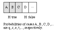
Proof. For definiteness, we suppose that the hypothesis in question is true in three cases as in the example. The argument differs inessentially for other examples, with other finite numbers of cases. Now consider the following array of tickets. Suppose I am willing to buy or sell any or all of these tickets at the stated prices. Why should p be the sum q+r+s?
Because no matter what it's worth -- $1 or $0 -- the ticket on H is worth exactly as much as the tickets on A, B and C together. (If H loses it's because A, B and C all lose; if H wins it's because exactly one of A, B, C wins.) Then if the price of the H ticket is different from the sum of the prices of the other three, I am inconsistently placing different values on one and the same contract, depending on how it is presented.
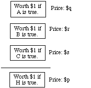
If I am inconsistent in that way, I can be fleeced by anyone who'll ask me to sell the H ticket and buy the other three (in case p is less than q+r+s) or buy the H ticket and sell the other three (in case p is more). Thus, no matter whether the equation p = q+r+s fails because the left-hand side is less than the right or more, a book can be made against me.
That's the Dutch book argument for additivity when the number of ultimate cases under consideration is finite. The talk about being fleeced is just a way of dramatizing the inconsistency of any policy in which the dollar value of the ticket on H is anything but the sum of the values of the other three tickets: to place a different value on the three tickets on A, B, C from the value you place on the H ticket is to place different values on the same commodity bundle under two demonstrably equivalent descriptions.
When the number of cases is infinite, a Dutch book argument for additivity can still be given -- provided the infinite number is not too big!
It turns out that not all infinite sets are the same size. The smallest infinite sets are said to be "countable." A countable set is one whose members can be listed: first, second, etc., with each member of the set appearing as the n'th item for some finite n. Of course any finite set is countable in this sense, and some infinite sets are countable. An obvious example of a countably infinite set is the set { 1, 2, 3, ... } of the positive whole numbers. A less obvious example is the set { ... , -2, -1, 0, 1, 2, ... } of all the whole numbers; it can be rearranged in a list (with a beginning): 0, 1, -1, 2, -2, 3, -3, ... . Then it is countable. Order doesn't matter, as long as they're all in the list. But there are uncountably infinite sets, too (example 3).
Example 2. In the election example, suppose there were an endless list of candidates, including no end of women. If H says that a woman wins, and A1, A2, etc., identify the winner as the first, second, etc. woman, then an extension of the finite additivity law to countably infinite sets would be as follows, with no end of terms on the right.
P(H) = P(A1) + P(A2) + ...
Thus, if the probability of a woman's winning were 1/2, and the probabilities of winning for the first, second, third, etc. woman were 1/4, 1/8, 1/16, etc. (decreasing by half each time), the equation would be satisfied.
Dutch book argument for additivity in the countably infinite case. Whatever my probabilities P(An) may be, if they don't add up to P(H) there will be an infinite set of $1 bets on truth of A1, A2, ... separately, on which my net gain will surely be the same as my gain from betting $1 on truth of H. (Note that this infinity of bets can be arranged by a finite contract: "In consideration of $1 paid in advance, Bookmaker hereby undertakes to pay Bettor the amount $P(the true one) when the true one has been identified.") This will be a Dutch book if the sum P(A1) + P(A2) + ... is greater or less than P(H)--against me if it's greater, against the bookmaker if it's less.
Summarizing, the following additivity law holds for any countable set of alternatives, finite or infinite.
Countable Additivity. If the possible cases are countable, the probability of a hypothesis is the sum of the probabilities of the cases in which it is true.
Example 3. Cantor's Diagonal Argument. The collection of all sets of positive whole numbers is not enumerable. For, given any list N1, N2, ... , there will be a "diagonal" set D consisting of the positive whole numbers n that do not belong to the the corresponding sets Nn in the list. For example, supose the first two entries in the list are N1 = the odd numbers = {1, 3, ...}, and N2 = the powers of 10 = {1, 10, ...}. Then it is false that D = N1, because 1 is in N1 but not in D; and it is false that D = N2, because 2 is in D but not in N2. (For it to be true that D = N2 it must be that each number is in both D and N2 or in neither.) In general, D cannot be anywhere in the list N1, N2, ... because by definition of D, each positive whole number n is in one but not the other of D and Nn.
The simplest laws of probability are the consequences of additivity under this assumption:
1.3 Laws of Probability
Probabilities are real numbers in the unit interval, 0 to 1, with the endpoints reserved for certainty of falsity and of truth, respectively.
This makes it possible to read laws of probability off diagrams, much as we read laws of logic off them.
Let's pause to recall how that works for laws of logic. Example:
De Morgan's Law. -(G&H) = -Gv-H
Here the symbols '-', '&' and 'v' stand for not, and, and or. Thus, if G is the hypothesis that the water is green, and H is the hypothesis that it's hot, then G&H is the hypothesis that it's green and hot, GvH is the hypothesis that it's green or hot (not excluding the possibility that it's both), and -G and -H are the hypothesis that it's not green, and not hot. Here is a diagram for De Morgan's law.

Stippled: -Gv-H
Points in such diagrams stand for the ultimate cases -- say, complete possible courses of events, each specified in enough detail to make it clear whether each of the hypotheses under consideration is true or false in it. The cases where G and H are both true are represented by points in the upper left-hand corner; that's the G&H region. The cases where at least one of G, H is true make up the GvH region, which covers everything but the points in the lower right-hand corner, where G and H are both false (-G&-H). And so on.
In general, the merger of two regions covers the cases where one hypothesis or the other is true, and the intersection of two regions covers the cases where both hypotheses are true.
Now in the diagram for De Morgan's law, above, the stippled region covers what's outside the G&H corner; then it represents the denial -(G&H) of G&H. At the same time it represents the merger (-Gv-H) of the lower region, where G is false, with the right-hand region, where H is false. So the law says: denying that G and H are both true, -(G&H), is the same as (=) asserting that G is false or H is, -Gv-H.
Adapting that sort of thing to probabilistic reasoning is just a matter of thinking of the probability of a hypothesis as its region's fraction of the area of the whole diagram. Of course the fraction for the whole Hv-H rectangle is 1, and the fraction for the empty H&-H region is 0. It's handy to be able to denote those two in neutral ways. Let's call them 1 and 0:
The Whole Rectangle: 1 = Hv-H = Gv-G etc.
The Empty Region: 0 = H&-H = G&-G etc.
Now let's read a couple of probability laws off diagrams.

Proof. The GvH area is the G area plus the H area, eacept that when you simply add, you count the G&H bit twice. So subtract it on the right-hand side.

Proof. The G&-H region is what remains of the G strip after you delete the G&H region.
We will often abbreviate by dropping ampersands (&), e.g., writing the subtraction law as follows.
Subtraction. P(G-H) = P(G)-P(GH)
Solving that for P(G), we have the rule of

In general, there is a rule of n-adic analysis for each n, e.g., for n=3:

You can verify the next two rules on your own, via diagrams.
Not. P(-D) = 1-P(D)
If. P(Hv-D) = P(DH)+P(-D)
In the second, 'H if D' is understood truth-functionally, i.e., as synonymous with 'H, unless not D': H or not D.

The idea is that saying "If D then H" is a guarded way of saying "H", for in case 'D' is false, the "if" statement makes no claim at all -- about "H" or anything else.
The next rule is an immediate consequence of the fact that logically equivalent hypotheses, e.g., -(GH) and -Gv-H, are always represented by the same region of the diagram.
Equivalence. Logically equivalent hypotheses are equiprobable.
That fact is also presupposed when we write '=' to indicate logical equivalence. Thus, since -(GH) = -Gv-H, the probability of the one must be the same as the probability of the other, for the one is the other.
Recall that to be implied by G, H must be true in every case in which G is true, not just in the actual case. (In other words, the conditional "H if G" must be valid: true as a matter of logic.) Then the G region must lie entirely inside the H region.This gives us the following rule.

Just as we identified your ordinary (unconditional) probability for H as the price you would think fair for the ticket at the left below, we now identify your conditional probability for H given D as the price you would think fair for the ticket at its right. We wrote 'P(H)' for the first of these prices. We write 'P(H | D)' for the second.
1.4 Conditional Probability

The tickets are represented as follows in diagrammatic form, with numbers indicating dollar values in the various cases.

The first ticket represents a simple bet on H; the second represents a conditional bet on H, i.e., a bet that's called off (the price of the ticket is refunded) in case the condition D fails. If D and H are both true the bet's on and you win; if D is true but H is false the bet's on and you lose; and if D is false, the bet's off: you get your $P(H | D) back.
With that understanding we can construct a Dutch book argument for the rule connecting conditional and unconditional probabilities:
Product Rule. P(DH) = P(D)P(H | D)
Imagine that your pockets are stuffed with money and tickets whose prices you think fair -- including the following three tickets. The first represents a conditional bet on H given D; the second and third represent unconditional bets on DH and against D, respectively. The third bet has an odd payoff, i.e., not a whole dollar, but only $P(H | D). That's why its price isn't the full $P(-D) but only the fraction P(-D) of the $P(H | D) that you stand to win. This third payoff was chosen to equal the price of the first ticket. That's what makes the three fit together into a neat book.
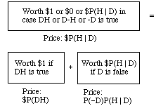
The three tickets are shown below in compact diagrammatic form. In each, the upper and lower halves represent D and -D, and the left and right halves represent H and -H. The number in each region shows the ticket's value when the corresponding hypothesis is true.

Observe that in every possible case regarding truth and falsity of D and H the second two tickets together have the same value as the first. Then there is nothing to choose between the first and the other two together, and so it would be inconsistent to place different values on them. Thus, the price you think fair for the first ought to equal the sum of the prices you think fair for the other two: P(H | D) = P(DH)+P(-D)P(H | D). Rewriting P(-D) as 1-P(D), this boils down to
P(H | D) = P(DH) + P(H | D) - P(D)P(H | D).
Cancelling the term on the left and the second term on the right and transposing, we have the product rule.
That's the Dutch book argument for the product rule: to violate the rule is to place different values on the same commodity bundle when it is described in two probably equivalent ways.
Here is the product rule in a slightly different form:
1.5 Laws of Conditional Probability
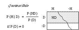
Graphically, the quotient rule expresses P(H | D) as the fraction of the area of the D strip that lies in the H region. It's as if calculating P(H | D) were a matter of trimming the square down to the D strip by discarding the blank region, and taking the stippled region as the new unit of area. Thus the conditional probability distribution assigns to H as its probability the H fraction of the D strip, the fraction P(HD)/P(D).
The quotient rule is often spoken of as a definition of conditional probability in terms of unconditional ones -- when the unconditional probability of the condition D is positive. But if P(D) is zero then by the implication rule so is P(DH), and the quotient P(DH)/P(D) assumes the indeterminate form 0/0. Then if the quotient rule really were its definition, the conditional probability would be undefined in all such cases. Yet, in many cases in which P(D)=0, we do assign definite values to P(H | D).
Example: the spinner. Although the probability is 0 that when the spinner stops it will point straight up (U) or straight down (D) we want to say that the conditional probability of up, given up or down,is 1/2: although P(U)/P(UvD) = 0/0, still P(U | UvD) = 1/2.
By applying the product rule to each term on the right-hand side of the analysis rule, P(D) = P(DH1) + P(DH2) + ..., we get the rule of
Total Probability
If the H's are incompatible and exhaustive,
P(D) = P(D|H1)P(H1) + P(D|H2)P(H2) + ...
Example. A ball will be drawn at random from urn 1 or urn 2, with odds 2:1 of being drawn from urn 2. Is black or white the more probable outcome?

Solution. By the rule of total probability with n=2 and D=black, we have
P(D) = P(D | H1)P(H1)+P(D | H2)P(H2) =
(3/4) (1/3)+(1/2) (2/3) =
1/4 + 1/3 = 7/12,i.e., a bit over 1/2. So black is the more probable outcome.
Finally, note that for any fixed proposition D of positive probability, the function P( | D) obeys all the laws of unconditional probability, e.g., additivity:
P(GvH | D) = P(G | D) + P(H | D) - P(G&H | D)
(Proof. Multiply both sides of the equation by P(D), and apply the product rule.) Therefore we sometimes write the function P( | D) as PD( ), e.g., in the additivity law:
PD(GvH) = PD(G) + PD(H)PD(-H) - PD(G&H)
If we condition again, on E, PD becomes PD&E:
PD(H | E) = PDE(H) = P(DEH)/P(DE) = P(H | DE)
The bar in 'P(H | D)' isn't a connective that turns pairs H, D of propositions into new, conditional propositions, H if D. Rather, it is as if we wrote the conditional probability of H given D as 'P(H, D)': the bar is a typographical variant of the comma. Thus we use 'P' for a function of one variable as in 'P(D)' and 'P(HD)', and also for the corresponding function of two variables as in 'P(H | D)'. The ambiguity is harmless because in every context, presence or absence of the bar clearly marks the distinction between the two uses. But of course the two are connected, i.e., by the product rule, P(HD) = P(H | D)P(D). That's why it's handy to make 'P' do double duty.
1.6 Why '|' Can't be a ConnectiveBut what is it that goes wrong when we treat the bar as a statement-forming connective, 'if'? This question was answered by David Lewis in 1976, pretty much as follows.
Consider the simple special case of the rule of total probability where there are only two hypotheses, H and -H:
P(X) = P(X | H). P(H) + P(X | -H). P(-H)
Now if '|' is a connective, H | D is a proposition, and we are entitled to set X = H | D above. Result:
(*) P(H | D) = P[(H | D) | H] P(H) + P[(H | D) | -H] P(-H)
So far, so good. But remember: '|' means if, so
'((H | D) | G)' means If G, then if D then H.
And as we ordinarily use the word 'if', this comes to the same as If D and G, then H:
(H | D) | G = H | DG
(The identity means that the two sides represent the same region, i.e., the two sentences are logically equivalent.) Now we can rewrite (*) as follows.
P(H | D) = P(H | DH). P(H) +
P(H | D-H). P(-H)
-- where the two terms on the right reduce to 1. P(H) and 0. P(-H), so that (*) itself reduces to
P(H | D) = P(H).
Conclusion: If '|' is a connective ("if"), conditional probabilities don't depend on their conditions at all. That means that 'P(H | D)' would be just a clumsy way of writing 'P(H)'. And it means that P(H | D) would come to the same thing as P(H | -D), and as P(H | G) for any other statement G. That's David Lewis's "trivialization result."
In proving this, the only assumption needed about "if" was that "If A, then if B then C" is equivalent to "If A and B then C": whatever region of a diagram represents (C | B) | A must also represent C | BA.
Back to the Index
Please write to bayesway@princeton.edu with any comments or suggestions.