Back to the Index
CHAPTER 3: EXPECTATION
Introduction
It was in terms of gambling that Pascal, Fermat, Huygens and others in their wake floated the modern probability concept. Betting was their paradigm for action under uncertainty; adoption of odds or probabilities was the relevant form of factual judgment. They saw probabilistic factual judgment and graded value judgment as a pair of hands to shape decision.
3.1 Desirability
The matter was put as follows in the final section of a most influential 17th century How to Think book, "The Port-Royal Logic" (1662)."To judge what one must do to obtain a good or avoid an evil, it is necessary to consider not only the good and the evil themselves, but also the probability that they happen, or not; and to view geometrically the proportion that all these things have together."
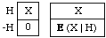
This "geometrical" view takes seriously the perennial image of deliberation as a weighing in the balance. Where a course of action might eventuate in a good or an evil, we are to weigh the probabilities of those outcomes in a balance whose arms are proportional to the gain and the loss that the outcomes would bring. To consider the "good and the evil themselves" is to compare their desirability differences, g-f and f-e in Fig. 1.
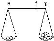
Fig. 1. Lengths are proportional to desirability differences, weights to probabilities. The desirability of the course of action is represented by the position f of the fulcrum about which the opposed turning effects of the weights just cancel.
Example 1. The last digit. The action under consideration is a bet on the last digit of the serial number of a $5 bill in your pocket: if it's one of the 8 digits from 2 to 9, you give me the bill; if it's 0 or 1, I give you $20. Then my odds on winning are 4:1. In the balance diagram, that's the ratio of weights in the pans. Suppose I have $100 on hand. Crassly, I might see my present desirability level as f = 100, and equate the desirabilities g and e with the cash I'll have on hand if I win and lose: g=105 and e=80. Now the 4:1 odds between the good and the evil agree with the 4:1 ratio of loss (f-e = 20) to gain (g-f = 5) as I see it. I'd think the bet fair.
In example 1, the options ("acts") were (G) take the gamble, and (-G) don't. My desirabilities des(act) for these were averages of my desirabilities des(level & act) for possible levels of wealth after acts, weighted with my probabilities P(level | act) for levels given acts:
des(G) = des($80 & G)P($80 | G) + des($105 & G)P($105 | G)
des(-G) = des($100 & -G)
If desirability equals wealth in dollars no matter whether it is a gain, a loss, or the status quo, these work out as:
des(G) = (80)(.25)+(100)(0)+(105)(.75) = 100
des(-G) = (80)(0)+(100)(1)+(105)(0) = 100
Then my desirabilities for the two acts are the same, and I am indifferent between them.
In the next example preference between acts reveals a previously unknown feature of desirabilities.
Example 2. The Heavy Smoker. The following statistics were provided by the American Cancer Society in the early 1960's.
                Percentage of American Men Aged 35
                  Expected to Die before Age 65
Nonsmokers                      23%
Cigar and Pipe Smokers          25%
Cigarette smokers:
  Less than 1/2 pack a day      27%
  1/2 to 1 pack a day           34%
  1 to 2 packs a day            38%
  2 or more packs a day         41%
In 1965, Diamond Jim, a 35-year-old American man, had found that if he smoked cigarettes at all, he smoked 2 or more packs a day. Thinking himself incapable of quitting altogether, he saw his options as the following two.C = Continue to smoke 2 or more packs a day S = Switch to pipes and cigarsAnd he saw these as the relevant conditions:L = He lives to age 65 or more D = He dies before the age of 65His probabilities came from the statistics in the normal way, so that, e.g., P(D | C) = 41% and P(D | S) = .25. Thus, his conditional probability matrix was as follows.L D C 59% 41% S 75% 25%Unsure of the desirabilities of the four conjunctions of C and S with D and L, he was clear that DS (= die before age 65 in spite of having switched) was the worst of them; and he thought that longevity and cigarette-smoking would contribute independent increments of desirability, say l and c:
des(LS) = des(DS)+l, des(LC) = des(DC)+l
des(LC) = des(LS)+c, des(DC) = des(DS)+c
Then if we set the desirability of the worst conjunction equal to d, his desirability matrix is this:
        L       D
C       d+c+l   d+c
S       d+l     d
Now in Diamond Jim's judgment the desirability of (C) continuing to smoke 2 packs a day and of (S) switching are as follows.
des(C) = des(LC)P(L | C) + des(DC)P(D | C)
= (d +c +l )(.59) + (d +c )(.41) = d +c +.59l
des(S) = des(LS)P(L | S) + des(DS)P(D | S)
= (d +l )(.75) + (d )(.25) = d +.75l
The difference des(C)-des(S) between these is c -.16l. If Diamond Jim preferred to continue smoking, this was positive; if he preferred swiching, it was negative.
Fact: Diamond Jim switched. Then the difference was negative, i.e., c was less than 16% of l: his preference for cigarettes over pipes and cigars was less than 16% as intense as his preference for living to age 65 or more over dying before age 65.
3.2 Problems
1 Train or Plane? With regard to cost and safety, train and plane are equally good ways of getting from Los Angeles to San Francisco. The trip takes 8 hours by train but only 1 hour by plane, unless the San Francisco airport proves to be fogged in, in which case the plane trip takes 15 hours. The weather forecast says there are 7 chances in 10 that San Francisco will be fogged in. If your desirabilities are simply negatives of travel times, how should you go?
2 The point of Balance. What must the probability of fog be, in problem 1, to make you indifferent between plane and train?
3 You assign the following desirabilities to wealth.
$: 0 10 20 30 40
des($): 0 10 17 22 26
a. With assets of $20 you are offered a gamble to win $10 with probability .58 or otherwise lose $10. Work out your desirabilities for accepting and rejecting the offer. Note that you should reject it.
b. What if you had been offered a gamble consisting of two independent plays of the gamble in (a)? Should you have accepted?
4 The Allais Paradox. You may choose one of the following options at no cost to yourself. Don't calculate, just decide!
A: One million dollars ($1M) for sure.
B: 10 or 1 or 0 $M with probabilities 10%, 89%, 1%.
What if you were offered the following options instead? Decide!
C: $1M or $0 with probabilities 11%, 89%.
D: $10M or $0 with probabilities 10%, 90%.
Note your intuitive answers; then compute your desirabilities for the four options, using x, y, z for the desirabilities of $10M, $1M, $0. Verify that the excess desirability of A over B in must be the same as that for C over D. Thus a policy of maximizing conditional expectation of dollar payoffs would have you prefer C to D if you prefer A to B.
5 The Ellsberg Paradox. A ball will be drawn from an urn containing 90 balls: 30 red, the rest black and yellow in some unknown ratio. As in problem 4, choose between A and B, and between C and D. Then calculate.
A: $100 if red, $0 if not. B: $100 if black, $0 if not.
C: $0 if red, $100 if not. D: $0 if black, $100 if not.
6 Deutero Russian Roulette. You've got to play Russian roulette, using a six-shooter that has 2 loaded cylinders. You've got a million, and would pay it all to empty both cylinders before you have to pull the trigger. Show that if dying rich is no better than dying poor, and it's the prospects of being dead, or being alive at various levels of wealth to which you attach your various desirabilities, the present decision theory would advise you to pay the full million to have just 1 bullet removed if originally there were 4 in the cylinder.
7 Proto Russian Roulette. If dying rich is no better than dying poor, and des(Dead)=0, des(Rich)=1, how many units of desirability is it worth to remove a single bullet before playing Russian Roulette when the six-shooter has e empty chambers?
8 In the Allais and Ellsberg paradoxes, and in Proto Russian Roulette, many people would choose in ways incompatible with the analyses suggested above. Thus, in problem 4, the desirability of being so unlucky as to win nothing in option B - having passed up the option (A) of a sure million - is often seen as much lower than the desirability of winning nothing in option C or D. Verify that the view of decision-making as desirability maximization needn't then see preference for A over B and for D over C as irrational.
Review the Allais and Ellsberg paradoxes in that light. (Note that in each case the question of irrationality is addressed to the agent's values, i.e., determinants of desirability, rather than to how the agent weighs those values together with with probabilities.)
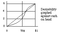
9 It takes a dollar to ride the subway. You and I each have a half-dollar coin, and sorely need a second. For each, desirabilities of cash are as in the graph above, so we decide to toss one coin and give both to you or to me depending on whether the head or tail turns up. In dollars, each thinks the gamble neither advantageous nor disadvantageous, since the expectation is 50cents , i.e., half way between losing ($0) and winning ($1). But in desirability, each thinks the gamble advantageous. To see why, read des(gamble) and (b) des(don't) off the graph.
10 The Certainty Equivalent of a Gamble
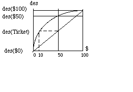
According to the graph, $50 in hand is more desirable than a ticket worth $100 or $0, each with probability 1/2, a ticket of "actuarial value" $50. How many dollars in hand would be exactly as desirable as the ticket?
11 The St. Petersburg Paradox.
"Peter tosses a coin and continues to do so until it should land "heads" when it comes to the ground. He agrees to give Paul one ducat if he gets "heads" on the very first throw, two ducats if he gets it on the second, four if on the third, eight if on th e fourth, and so on, so that with each additional throw the number of ducats he must pay is doubled. Suppose we seek to determine the value of Paul's expectation."
Paul's probability that the first head comes on the n'th toss is pn = 1/2n, and in that case Paul's receipt is rn = 2n-1. Then Paul's expectation of gain, p1r1+p2r2+..., will be 1/2+1/2+... = *. Then should Paul be glad to pay any finite sum for the privilege of playing?
"This seems absurd because no reasonable man would be willing to pay 20 ducats as equivalent. You ask for an explanation of the discrepancy between the mathematical calculation and the vulgar evaluation. I believe that it results from the fact that, in their theory, mathematicians evaluate money in proportion to its quantity while, in practice, people with common sense evaluate money in proportion to the utility they can obtain from it."
If the desirability des(r) of receiving r ducats increases more and more slowly, des(gamble) might be finite:
des(gamble) = des(r1)/2 + des(r2)/4 + ... + des(rn)/2n + ...
"If, for example, we suppose the moral value of goods to be directly proportionate to the square root of their mathematical quantities, e.g., that the satisfaction provided by 40,000,000 is double that provided by 10,000,000, my psychic expectation becomes
1/2+
On this reckoning Paul should not be willing to pay as much as 3 ducats to play the game, for des(3) is
But the paradox reappears as long as des(r) does eventually exceed any preassigned value, for then a variant of the St. Petersburg game can be devised in which the payoffs rn are large enough so that des(r1)p1 + des(r2)p2 + ... =
.
Problem. With des(r) =
3.3 Rescaling
A balanced beam would remain balanced if expanded or contracted uniformly about the fulcrum, e.g., if each inch stretched to a foot, or shrank to a centimeter. That's because balance is a matter of cancellation of the net clockwise and counterclockwise turning effects, and uniform expansion or contraction would multiply each of these by a common factor k, e.g., k=12 if inches stretch to feet and k=.3937 if inches shrink to centimeters.Applying the laws of the lever to choice, we conclude that nothing relevant to decision-making depends on the size of the unit of the desirability scale.
Furthermore, nothing relevant to decision-making depends on the location of the zero of the desirability scale. In physics this corresponds to the fact that if a beam is in balance then the turning effects of the various forces on it about any one point add up to 0, whether or not the point is the fulcrum - provided we view the fulcrum as pressing upward with a force equal to the net weight of the loaded beam
Then if numbers des(H) accurately represent your judgments of how good it would be for hypotheses H to be true, so will the numbers ades(H), where a is any positive constant. That's because multiplying by a positive constant is just a matter of uniformly shrinking or stretching the scale -- depending on whether the constant is greater or less than 1 (as when lengths in feet look 12 times as great in inches and 1/3 as great in yards). And if numbers des(H) accurately represent your valuations, so will ades(H)+b, where a is positive and b is any constant at all; for moving the origin of coordinates left (positive b) or right (negative b) by the same amount, b, leaves distances between them (gains and losses) unchanged.
E.g., in example 13.2, we can set d=0, l=1 without thereby making any substantive assuptions about Diamond Jim's desirabilities. On that scale, desirabilities of the acts are simply des(C) = c + .59 and des(S) = .75.
Two desirability assignments des and V determine the same preferences among options if the graph of one against the other is a straight line des' (H) = ades(H)+b as in Fig. 1, sloping up to the right, so that des' is a positive linear transform of des. The multiplicative constant a is the line's slope (rise per unit run); the additive constant b is the des'-intercept, the height at which the line cuts the des'-axis.
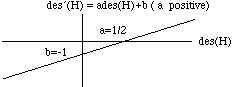
Fig. 1. des and des' are equivalent desirability scales.
There is less scope for rescaling probabilities. If the weights in all pans are multiplied by the same positive constant, balance will not be disturbed; but no other sort of change, e.g., adding the same extra weight to all pans, can be relied upon never to unbalance the scales.
It would be all right to use different positive numbers as probabilities of a sure thing in different problems -- perhaps, the upward force at the fulcrum. Although do use 1 as the probability of a sure thing in every problem, that is just a convention; any positive constant would do.
On the other hand, we adopt no such convention for desirabilities, e.g., we do not insist that the desirability of a sure thing (Av-A) always be 0, or that the desirability of an impossibility (A&-A) always be 0.
3.4 Expectations, RV's, Indicators
My expectation of any unknown quantity -- any so-called "random variable" (or "RV" for short) -- is a weighted average of the values I think it can assume, in which the weights are my probabilities for those values.
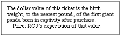
Example 1. Giant Pandas. Let X = the birth weight to the nearest pound of the next giant panda (ailuropoda melanoleuca) to be born in captivity. If I have definite probabilities p0, p1, etc. for the hypotheses that X = 0, 1, ... , 99, etc., my expectation of X will be
0. p0 + 1. p1 + ... +99. p99 + ...
This sum can be stopped after the 99th term without affecting its value, since I attribute probability 0 to values of X of 100 or more.
It turns out that probability itself is an expectation:
Indicator Property. My probability p for truth of a hypothesis is my expectation of a random variable (the "indicator" of the hypothesis) that has value 1 or 0 depending on whether the hypothesis is true or false.
Proof. As 1 and 0 are the only values this RV can assume, its expectation is 1p + 0(1-p), i.e., p.
Observe that an expected value needn't be one of the values the random variable can actually assume. Thus in the Panda example X must be a whole number; but its expected value, which is an average of whole numbers, need not be a whole number. Nor need my expectation of the indicator of past life on Mars be one of the values that indicators can assume, i.e., 0 or 1; it might well be 1/10, as in the story at the beginning of chapter 1.
The indicator property of expectation is basic. So is this:
Additivity. Your expectation of a sum is
the sum of your expectations of its terms.
From additivity it follows that your expectation of X+X is twice your expectation of X, your expectation of X+X+X is three times your expectation of X, and for any whole number n,
Proportionality. Your expectation of
nX is n times your expectation of X.
Example: 2. Success Rates. I attribute the same probability, p, to success on each trial of an experiment. Consider the indicators of the hypotheses that the different trials succeed. The number of successes in the first n trials will be the sum of the first n indicators; the success rate in the first n trials will be that sum divided by n. Now by additivity, my expectation of the number of successes must be the sum of my expectations of the separate indicators. Then by the indicator property, my expectation of the number of successes in the first n trials is np. Therefore my expectation of the success rate in the first n trials must be np divided by p, i.e., p itself.
That last statement deserves its own billing:
Calibration Theorem. If you have the same probability (say, p) for success on each trial of an experiment, then p will also be your expectation of the success rate in any finite set of trials.
The name comes from the jargon of weather forecasting; forecasters are said to be well calibrated when the fraction of truths ("success rate") is p among statements to which they have attributed p as probability. Thus theß theorem says: forecasters expect to be well calibrated.
3.5 Why Expectations are Additive
Like probabilities, expectations can be related to prices. My expectation of a magnitude X can be identified with the buying-or-selling price I'd think fair for a ticket that can be cashed for X(r) units of currency. A ticket for X as in the Panda example is shown above. By comparing prices and values of combinations of such tickets we can give a Dutch book argument for additivity of expectations.
Suppose x and y are your expectations of magnitudes X and Y -- say, rainfall in inches during the first and second halves of next year -- and z is your expectation for next year's total rainfall, X+Y. Why should z be x+y?
Because in every eventuality about rainfall at the two locations, the first two of these tickets together are worth the same as the third:
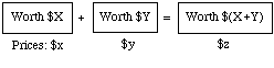
Then unless the prices you would pay for the first two add up to the price you would pay for the third, you are inconsistently placing different values on the same prospect, depending on whether it is described to you in one or the other of two provably equivalent ways.
3.6 Conditional Expectation
Just as we defined your conditional probabilities as the prices you'd think fair for tickets that represent conditional bets, so we define conditional expectations:
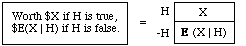
Your conditional expectation E(X | H) of the random variable X given truth of the statement H is the price you'd think fair for the following ticket:
Corresponding to the notation E(X | H) for your conditional expectation for X, we use E(X) for your unconditional expectation for X, and E(XY) for your unconditional expectation of the product of the magnitudes X and Y.
The following rule might be viewed as a definition of conditional expectations in terms of unconditional ones in case P(H)!= 0, just as the quotient rule for probabilities might be viewed as a definition of P(G|H) as the quotient P(G&H)/P(H). On the right-hand side, IH is the indicator of H. Therefeore P(H)=E(IH).
Quotient Rule.
E(X | H) = E(X. IH)/P(H)
The quotient rule is equivalent to the following relationship between conditional and unconditional expectations.
Product Rule.
E(X. IH) = E(X | H)P(H)
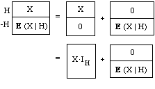
A "Dutch book" consistency argument for this relationship can be modelled on the one given in sec. 4 of for the corresponding relationship between probabilities. Consider the following tickets. Clearly, the first has the same value as the pair to its right, whether H is true or false. And those two have the same values as the ones under them, for XIH is X if H is true and 0 if H is false, and the last ticket just duplicates the one above it. Then unless your price for the first ticket is the sum of your prices for the last two, i.e., unless the condition
E(X | H) = E(X. IH) + E(X | H)P(-H),
is met, you are inconsistently placing different values on the same prospect depending on whether it is described in one or the other of two provably equivalent ways. Now set P(-H) = 1-P(H) in this condition, and simplify. It boils down to the product rule.
Historical Note. Solved for P(H), the product rule determines H's probability as the ratio of E(X. IH) to E(X | H). As IH is the indicator of H, X. IH is X or 0 depending on whether H is true or false. Thus, viewed as a statement about P(H), the product rule corresponds to Thomas Bayes's definition of probability:
"The probability of any event is the ratio between the value at which an expectation depending on the happening of the event ought to be computed, and the value of the thing expected upon its happening."
E(X. IH) is the value you place on the ticket at the left; E(X | H) is the value you place on the ticket at the right:
The first ticket is "an expectation depending on the happening of the event", i.e., an expectation of $X depending on the truth of H, an unconditional bet on H.Your price for the second ticket, $E(X | H), is "the value of the thing expected [$X] upon its [H's] happening": as you get the price back if H is false, your uncertainty about H doesn't dilute your expectation of X here, as it does if the ticket is worthless when H is false.
3.7 Laws of Expectation
The basic properties of expectation are the product rule and
Linearity. E(aX+bY+c) = aE(X)+bE(Y)+c
Three notable special cases of the linearity equation are obtained by setting a=b=1 and c=0 (additivity), b=c=0 (proportionality), and a=b=0 (constancy):
Additivity. E(X+Y)=E(X)+E(Y)
Proportionality. E(aX)=aE(X)
Constancy. E(c)=c
By repeated application, the additivity equation can be seen to hold for arbitrary finite numbers of terms -- e.g., for 3 terms, by applying 2-term additivity to X+(Y+Z):
E(X+Y+Z) = E(X)+E(Y)+E(Z)
The magnitudes of which we have expectations are called "random variables" since they may have various values with various probabilities. May have: in the linearity property, a, b, and c are constants, so that, as we have seen, E(c) makes sense, and equals c. But more typically, a random variable might have any of a number of values as far as you know. Convexity says that your expectation for the variable cannot be larger than all of those values, or smaller than all of them:
Convexity. E(X) lies in the range from the
largest to the smallest values that X can assume.
Where X can assume only a finite numer of values, convexity follows from linearity.
The following connection between conditional and unconditional expectations is of particular importance. Here, the H's are any hypotheses whatever.
Total Expectation. If no two of H1, H2, ...
are compatible, and H is their disjunction, then
E(X | H) = E(X | H1)P(H1| H) + E(X | H2)P(H2| H)+ ...
Proof. X . IH = X . IH1 + X . IH2 + ... ; apply E to both sides, then use additivity and the product rule. Divide both sides by P(H), and use the fact that P(Hi)/P(H) = P(Hi| H) since Hi&H = Hi.
Note that when when conditions are certainties, conditional expectations reduce to unconditional ones:
Certainty. E(X | H) = E(X) if P(H)=1
Applying conditions. It is always OK to apply conditions of form Y = blah (e.g., Y = 2X) appearing at the right of the bar, to rewrite Y as blah at the left:
E(... Y... | Y=blah) = E(... blah... | Y=blah) (OK!)
The Discharge Fallacy. But we cannot generally discharge a condition Y=blah by rewriting Y as blah at the left and dropping the condition; e.g., E(3Y2 | Y=2X) cannot be relied upon to equal E(3(2X)2). In general:
E(... Y... | Y=blah) = E(... blah... ) (NOT!)
The problem of the two sealed envelopes. One contains a check for an unknown whole number of dollars, the other a check for twice or half as much. Offered a free choice, you pick one at random. You might as well have chosen the other, since you think them equally likely to contain the larger amount. What is wrong with the following argument for thinking you have chosen badly? "Let X and Y be the values of the checks in the one and the other. As you think Y equally likely to be .5X or 2X, E(Y) will be .5E(.5X) + .5E(2X) = 1.25E(X), which is larger than E(X)."
A Valid Special Case of the Discharge Fallacy.As an unrestricted rule of inference, the discharge fallacy is unreliable. (That's what it is, to be a fallacy.) But it becomes a valid rule of inference when "blah" represents a constant, e.g., as in "Y=.5". Show that the following is valid.
E(... Y... | Y=constant) = E(... constant... )
3.8 Physical Analogies; Mean and Median
Hydraulic Analogy. Let "F" and "S" mean heads on the first and second tosses of an ordinary coin. Suppose you stand to gain a dollar for each head. Then your net gain in the four possibilities for +/- F and +/- S will be as shown at the left below.
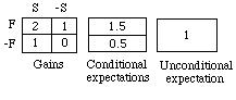
Think of that as a map of flooded walled fields in a plain, with the numbers indicating water depths in the four sections. In the four regions, depths are values of X and areas are probabilities. To find your expectation for X, open sluices so that the water reaches a common level in all sections. That level will be E(X). To find your conditional expectation for X given F, open a sluice between the two sections of F so that the water reaches a single level in F. That level will be E(X | F), i.e., 1.5. Similarly, E(X | -F) = 0.5. To find your unconditional expectation of gain, open all four sluices so that the water reaches the same level throughout: E(X) = 1.
There is no mathematical reason for magnitudes X to have only a finite numbers of values, e.g., we might think of X as the birth weight in pounds of the next giant panda to be born in captivity -- to no end of decimal places of accuracy, as if that meant something. (It doesn't. The commonplace distinction between panda and ambient moisture, dirt, etc. isn't drawn finely enough to let us take the remote decimal places seriously.) We can extend the hydraulic analogy to such continuous magnitudes by supposing that the fields may be pitted and contoured so that water depth (X) can vary continuously from point to point. But cases like temperature, where X can also go negative, require more tinkering -- e.g., solid state H2O, with heights on the iceberg representing negative values.
Balance. The balance analogy (sec. 13, Fig. 1) is more easily adapted to the continuous case. The narrow rigid beam itself is weightless. Positions on it represent values of a magnitude X that can go negative as well as positive. Pick a zero, a unit, and a positive direction on the beam. Get a pound of modelling clay, and distribute it along the beam so that the weight of clay on each section represents the probability that the true value of X is in that section. (Fig. 1 below is an example -- where, as it happens, X cannot go negative.)
Example. "The Median isn't the Message" In 1985 Stephen Gould wrote: "In 1982, I learned I was suffering from a rare and serious cancer. After surgery, I asked my doctor what the best technical literature on the cancer was. She told me ... that there was nothing really worth reading. I soon realized why she had offered that humane advice: my cancer is incurable, with a median mortality of eight months after discovery."
In terms of the balanced beam analogy, here are the key definitions, of the terms "median" and "mean" -- the latter being a synonym for "expectation":
The median is the point on the beam that divides the weight of clay in half: the probabilities are equal that the true value of X is represented by a point to the right and to the left of the median.
The mean (= your expectation ) is the point of support at which the beam would just balance.
Gould continues: "The distribution of variation had to be right skewed, I reasoned. After all, the left of the distribution contains an irrevocable lower boundary of zero (since mesothelioma can only be identified at death or before). Thus there isn't much room for the distribution's lower (or left) half -- it must be scrunched up between zero and eight months. But the upper (or right) half can extend out for years and years, even if nobody ultimately survives."
See Fig. 1, below. Being skewed (stretched out) to the right, the median of this probability distribution is to the left of its mean; Gould's life expectancy is greater than 8 months. (The mean of 24 months suggested in the graph is my invention. I don't know the statistics.)
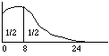
Fig. l. Locations on the beam are months lived after diagnosis; the weight of clay on the interval from 0 to m is the probability of still being alive in m months.
The effect of skewness can be seen especially clearly in the case of discrete distributions like the following. Observe that if the right-hand weight is pushed further right the mean will follow, while the median stays fixed. The effect is most striking in the case of the St. Petersburg game, where the median gain is between 1 and 2 ducats but the expected (mean) gain is infinite.
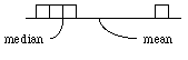
Fig. 2. The median stays between the second and third blocks no matter how far right you move the fourth block.
3.9 Desirabilies as Expectations
Desirability is a mixture of judgments of fact and value; your desirability for H represents a survey of your desirabilities for the various ways you think H could happen, combined into a single figure by multiplying each number by your probability for its being the desirability of the way H actually happens. In effect, your desirability for H is your conditional expectation of a magnitude ("U"), commonly called "utility":
des(H) = E(U | H)
U(s) is your desirability for a complete scenario, s, that says exactly how everything turns out. Then U(s) records a pure value judgment, untainted by uncertainty about details, whereas des(H) mixes pure value judgments with pure factual judgments.
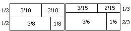
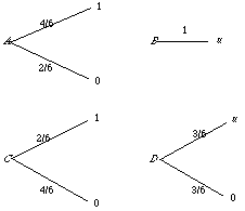
Example 1. The Heavy Smoker, Again (cf. example 13.2). In Fig.1(a), U's actual value is the depth of the unknown point representing the real situation, and desirabilities are average depths -- e.g., the desirability des(SL)=1 of switching and living at least 5 more years is a probability-weighted average of all manner of ways for that to happen--hideous, delightful, or middling. With P(L | C)=.60 (nearly; it's really .59), and P(L | S) = .75, switching raises the odds on L:D from 3:2 to 3:1. Then in (b), desirabilities des(C)=.69 and des(S)=.75 are mixtures--of 1.1 with 1 in the ratio 3:2, and 1 with 0 in the ratio 3:1.
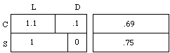
(a) des(act & outcome) (b) des(act)
Fig. 1. Hydraulic Analogy
(a) Initial P(act & outcome) (b) Final P(act & outcome)
Fig. 2. Unconditional probabilities. (Depths as in Fig. 1.)
Figures 1(a, b) and 2(a) are drawn with P(C) = P(S) = 1/2; the upper and lower sections have equal areas. That is one way to represent Diamond Jim's initial state of mind, unsure of his action. Another is to say he has no numbers at all in mind for P(C) and P(S), even though he does for P(L | C) and P(L | S). Either way, he has clearly not yet made up his mind, for when he has, P(C) and P(S) will be numbers near the ends of the unit interval. In fact, deliberation ends with a realization that switching has the higher desirability; he decides to make S true, or try to; final P(S) will be closer to 1 than initial P(S), i.e., 2/3 instead of 1/2 in Fig. 2. (Diamond Jim is far from sure he will carry out the chosen line of action.)
Warning. des(act) measures choiceworthiness only if odds on outcomes conditionally on acts remain constant as odds on acts vary -- e.g. as in Fig. 2, where odds on L:D given C and given S remain constant at 3:2 and 3:1 as odds on C:S vary from 1:1 to 1:2.
This warning is important in "Newcomb" problems, i.e., quasi-decision problems in which acts are seen as mere symptoms of outcomes that agents would promote or prevent if they could.
Example 2. Genetic Determinism. Suppose Diamond Jim attributes the observed correlations between smoking habits and longevities to the existence in the human population of two alleles (good, bad) of a certain gene, where the bad allele promotes heavy cigarette smoking and early death, and works against switching. Jim thinks it's the allele, not the habit, that's good or bad for you; he sees his act and his life expectancy as conditionally independent given his allele -- whether good or bad. And he sees the allele as hegemonic (sec. 11), determining the chances
P(act | allele), P(outcome | allele)
of acts and outcomes. Then higher odds on switching are a sign that his allele is the longevity-promoting one. He sees reason to hope to try to switch, but no reason to try.
3.10 Notes
Sec. 3.1 For the statistics in example 2, see The Consumers Union Report on Smoking and the Public Interest (Consumers Union, Mt. Vernon, N.Y., 1963, p. 69). This example is adapted from R. C. Jeffrey, The Logic of Decision (2nd ed., Chicago: U. of Chicago Press, 1983).
Sec. 3.2, Problems
1 and 2 come from The Logic of Decision.
3 is from D. V. Lindley, Making Decisions (New York: Wiley-Interscience, 1971), p. 96.
4 is from Maurice Allais, "Le comportment de l'homme rationnel devant la risque," Econometrica 21(1953): 503-46. Translated in Maurice Allais and Ole Hagen (eds.), Expected Utility and the Allais Paradox, Dordrecht: Reidel, 1979.
5 is from Daniel Ellsberg, "Risk, Ambiguity, and the Savage Axioms," Quarterly Journal of Economics 75(1961) 643-69.
6 is Alan Gibbard's variation of problem 7 (i.e. Richard Zeckhauser's) that Daniel Kahneman and Amos Tversky report in Econometrica 47 (1979) 283. See also "Risk and human rationality" by R. C. Jeffrey, The Monist 70(1987)223-236.
9. In the diagram, "marginal desirability" (rate of increase of desirability) reaches a maximum at des = 4, and then shrinks to a minimum at des = 6. The second half dollar increases des twice as much as the first.
11, The St. Petersburg paradox. Daniel Bernoulli's "Exposition of a new theory of the measurement of risk" (in Latin) appeared in the Proceedings of the St. Petersburg Imperial Academy of Sciences 5(1738) Translation: Econometrica 22 (1954) 123-36, reprinted in Utility Theory: A Book of Readings, ed. Alfred N. Page (New York: Wiley, 1968) The three quotations areare from correspondence between Daniel's uncle Nicholas Bernoulli and (first, 1713) Pierre de Montmort, and (second and third, 1728) G abriel Cramer.
It seems to have been Karl Menger (1934) who first noted that the paradox reappears as long as U(r) is unbounded; see the translation of that paper in Essays in Mathematical Economics, Martin Shubik (ed.), Priceton U. P., 1967, especially the first footnote on p. 211.
Sec. 3.4. For more about calibration, etc., see Morris DeGroot and Stephen Fienberg, "Assessing Probability Assessors: Calibration and Refinement," in Shanti S. Gupta and James O. Berger (eds.), Statistical Decision Theory and Related Topics III, Vol. 1, New York: Academic Press, 1982, pp. 291-314.
Sec. 3.5, 3.6. The Dutch book theorems for expectations and conditional expectations are bits of Bruno de Finetti's treatment of the subject in vol. 1 of his Theory of Probability, New York: Wiley, 1974.
Sec. 3.6. Bayes's definition of probability is from his "Essay toward solving a problem in the doctrine of chances," Philosophical Transactions of the Royal Society 50 (1763), p. 376, reprinted in Facsimiles of Two Papers by Bayes, New York: Hafner, 1963.
Sec. 3.8. "The Median isn't the Message" by Stephen Jay Gould) appeared in Discover 6(June 1985)40-42.
Sec. 3.9, example 2. This is a "Newcomb" problem; see Robert Nozick, "Newcomb's Problem and Two Principles of Choice" in Essays in Honor of Carl G. Hempel, N. Rescher, ed. (Dordrecht: Reidel Publishers, 1969). For recent references and further discussion, see Richard Jeffrey, "Causality in the Logic of Decision" in Philosophical Topics 21 (1993) 139-151.
SOLUTIONS
Sec. 3.2
1 Train 2 1/2 3(b) Yes.
5 If you prefer A to B, you should prefer D to C.
6 With 0 = des[die], 1 = des[rich and alive], and u = des[a million dollars poorer, but alive], suppose that u = des[get rid of the two bullets]; you'd pay everything you have. Then you are indifferent between A and B below.
To see that you must be indifferent between C and D as well, observe that if you plug the A diagram in at the "u" position in the D diagram, you get the DA diagram. But there, the probability of getting 1 is 1/3 (i.e., 1/2 times 2/3), so the probability of getting 0 one way or the other must be 2/3, and the DA diagram is equivalent to the C diagram. Thus you should be indifferent between C and D if you are indifferent between A and B.

7 1/(e+1) 9
(gamble) = 3,
10 $10 11 rn = (2n)2
Sec. 3.7, The Two Envelopes. It's the discharge fallacy. To see why, apply the law of total expectation and the assumption that P(Y=.5X) = P(Y=2X) = 1/2, to get this:
E(Y) = .5E(Y | Y=.5X) + .5E(Y | Y=2X)
By the discharge fallacy, we would then have
E(Y) = .5E(.5X) + .5E(2X) = 1.25E(X) (NOT!)
But in fact, what we have is this:
E(Y) = .5E(.5X | Y=.5X) + .5E(2X | Y=2X)
= .25E(X | Y=.5X) + E(X | Y=2X)
In fact, E(X) and E(Y) are the same mixture of your larger and smaller expectations of X when Y is the larger (2X) or smaller (X/2) amount: E(X) = E(Y) = five parts of E(X | Y=.5X) with two parts of E(X | Y=2X).
Back to the Index
Please write to bayesway@princeton.edu with any comments or suggestions.